Reproducible models · Tutorial 13 of 13
Reproducing Spatial Information Explained
A complete walkthrough of SIE — a validation metric that asks how much of the spatial information in a response a prediction model explains, not only how small its errors are: the spatial information of the response and of its block cross-validation residuals is measured with mutual information at several grid resolutions, and the relative reduction is aggregated with information weights. From a 4 × 4 example you can check by hand to the paper's ten-model case study across Australia, with every figure regenerated by one command.
To cite the SIE method and its codes in publications, please use:
Song Y (2026). Spatial information explained by prediction models under block cross-validation. ISPRS Journal of Photogrammetry and Remote Sensing 242:984–1000. doi · PDF · GitHub
sie.R (the SIE function, base R) · example.R (the case study) · c4-data.csv · reference-results.csv — all four unchanged from the GitHub repository — plus worked-example.R, further-analyses.R, run-all.R, the results/ and figures/ of a verified run, and a README.md. Unzip and run Rscript run-all.R from the sie/ folder.
The code published with the paper: sie() in a single base-R file, the C4 grass data for 2,480 grid cells across Australia, and example.R, which rebuilds the ten-model comparison and checks it against the reference results (GPL-3.0). SIE has no online calculator; sie() runs on any vector of out-of-fold predictions.
1 Method Overview & Reproduction Scope
1.1 Core Idea
A spatial prediction model is usually judged by RMSE or R²: how far its predictions are from the observations, averaged over the study area. Those numbers do not say whether the model has captured the geography of the response. Two models with the same RMSE can leave very different residuals — one spatially random, the other still organised into regional clusters, gradients or zones of unequal spread. Spatial information explained (SIE) measures that difference directly.
SIE treats spatial information as a measurable quantity: the mutual information I(Y; S) between a variable and its location, i.e. how much knowing where an observation is reduces the uncertainty about its value. A model that learns the spatial structure of the response leaves residuals that carry little of it. SIE is the relative reduction from the response to the residuals, E = 1 − I(ε; S) / I(Y; S), computed from out-of-fold residuals of spatial block cross-validation and aggregated over several grid resolutions.
- Research problem: validation metrics quantify error, not explained spatial structure; residual diagnostics such as Moran's I detect remaining dependence but not its share of the total; and existing spatial validation metrics are computed under random cross-validation, where nearby observations leak between training and test sets.
- One-line contribution: a normalised metric of explained spatial information — block-CV residuals + mutual information of the response and the residuals with location + a softmax-weighted multi-scale aggregate that needs no scale to be chosen.
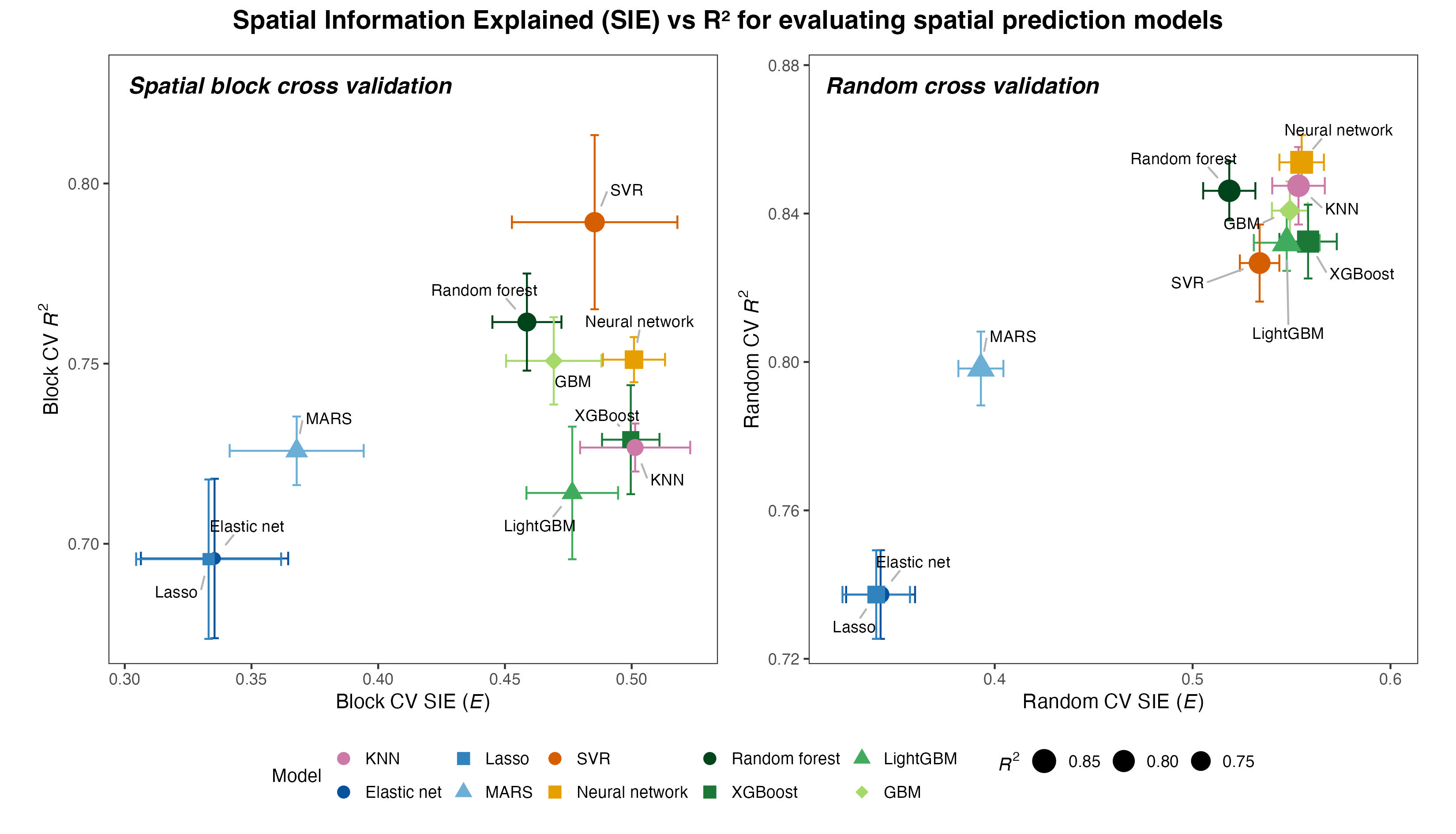
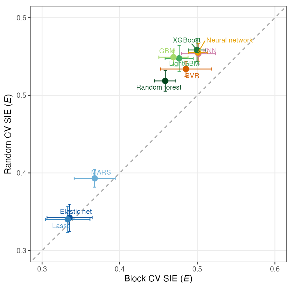
- Why it matters here: across ten models, SIE rankings differ from accuracy rankings (Spearman ρ = −0.38 with RMSE, 0.53 with R²): random forest has the second-lowest RMSE but ranks seventh in E. Random cross-validation overstates E for all ten models, by 2.1–17.0 % (mean 9.9 %). This tutorial regenerates all of it from the published code.
block CV → out-of-fold residuals ε = Y − ŶOOF → discretize (Y and ε into equal-frequency bins, location into a grid) → spatial information of the response I(Y; S) and of the residuals I(ε; S) → scale-specific Er → softmax weights from Ir(Y; S) → multi-scale E. Everything on this page serves that line.
R 4.1+. The metric itself, sie(), is one base-R file with no package dependency.
The case study adds the modelling packages of the paper (tidymodels and ten learner engines) and two
plotting helpers. All data ship with the code, so nothing is downloaded at run time. A full run takes
about 45 seconds.
1.2 Method Logic
SIE is computed in five steps. The notation follows the paper's Section 2 and the equation numbers are the paper's; every step is exercised by the pipeline in §3.
ε = Y − ŶOOF
nb bins × g × g grid
I(Y;S), I(ε;S)
Er at each grid
softmax weights → E
Step 1 — residuals from spatial block cross-validation
The study area is divided into contiguous blocks that are randomly assigned to k folds. Each fold is predicted by a model trained on the other folds, and the held-out predictions are concatenated into ŶOOF, aligned with Y. Residuals from a model fitted on all the data would overstate SIE, because spatial autocorrelation lets training points inform predictions at nearby locations.
Step 2 — discretization
Y and ε are each cut into nb equal-frequency bins at their empirical quantiles, which makes the entropy robust to skewed distributions. Location is discretized jointly: the bounding box of the data is split into a regular g × g grid and every observation takes the label of its cell. Empty cells carry no probability and are dropped; ns is the number of occupied cells.
Step 3 — spatial information as mutual information
Spatial information is the reduction in uncertainty about Y that comes from knowing its spatial unit, estimated from the discrete joint distribution in nats:
The same estimator applied to the residuals gives I(ε; S), the spatial information the model leaves behind. Mutual information reacts to any difference between the distribution inside a cell and the overall distribution — in mean, spread, skewness or tails — so it detects, for example, residuals whose variance changes across space even when their mean and autocorrelation do not.
Step 4 — SIE at one grid resolution
E = 1: the residuals hold no spatial information left; E = 0: the model has not reduced it (for a no-model baseline ε = Y, so E = 0 exactly). Values below zero, when residuals carry more spatial information than the response, are set to zero and signal misspecification. Mutual information is not additive, so E is a relative reduction, not a share of a fixed quantity split between model and residuals.
Step 5 — multi-scale SIE with information weights
Spatial dependence acts at several scales, so Er is evaluated on a set of grids {r1, …, rK} and combined with weights from the softmax of the response's spatial information at each scale (τ = 1):
The weights depend on Y only, so every model is scored with the same weights and no scale is picked by looking at model performance — picking the resolution that maximises Er would bias SIE upwards.
| Quantity | Symbol | In sie() | How to read it |
|---|---|---|---|
| Spatial information of the response | Ir(Y; S) | I_Y_S | how strongly location predicts the value of Y at grid r; grows as the grid is refined, so only comparable at a fixed grid |
| Residual spatial information | Ir(ε; S) | I_e_S | spatial structure the model has left in its errors |
| Scale-specific SIE | Er | E_r | relative reduction at one grid; a diagnostic profile |
| Information weight | wk | weight | softmax of Ir(Y; S); a peaked profile means one dominant grain, a flat one several |
| Multi-scale SIE | E | E | the reported metric, between 0 and 1 |
| Leading estimation bias | (nb − 1)(ns − 1) / 2n | bias | the positive bias of the plug-in estimate; keep it small relative to I(Y; S) (at most about 0.25 of it in the case study) |
The quantities of SIE and the columns of the scale profile that sie() returns.
The common bias inflates both mutual informations, which pulls E down: SIE is conservative, and at a
fixed resolution the bias is the same for every model, so it does not change their ranking.
1.3 The Two Experiments — Purpose, Results, Interpretation
The paper validates SIE on a simulation with known amounts of spatial learning, then applies it to ten machine learning models on real data. This tutorial re-runs the case study; the simulation is shown from the published article for reference.
Experiment 1 — simulation with a controlled learning ladder
| Purpose | check that E behaves as theory says: 0 when there is no spatial information or none is learned, rising monotonically as more of the spatial signal is learned |
|---|---|
| Data | a five-component spatial signal f(S) on the unit square plus Gaussian noise; predictions Ŷ = λ f(S) with λ from 0 to 1 |
| Settings | nb = 20 bins, one 8 × 8 grid; robustness over 14 configurations in four families (autocorrelation range, sample size, sampling pattern, noise type), 20 replicates each |
In the paper, E is zero both without spatial structure and when structure is present but not learned, and rises monotonically with the learned proportion of the signal in every configuration. Full learning stops at about 0.80 rather than 1: with residuals that are pure noise, the plug-in estimate of I(ε; S) is still positive — the finite-sample noise floor of the estimator, close to the leading bias term — so the ceiling of E depends on the bins, the grid and the sample size. The simulation is not part of this tutorial; its design and results are summarised in the SIE article.
Experiment 2 — C4 grass area across Australia, ten models
| Purpose | show that SIE separates models by the spatial information they explain, and how this relates to accuracy and to the cross-validation design |
|---|---|
| Data | 2,480 cells of 0.5° (2019): C4 natural grass area percentage, with the AC4/AC3 photosynthetic advantage ratio, mean annual temperature and mean annual precipitation as predictors |
| Models | random forest, XGBoost, LightGBM, GBM, SVR, a neural network (mean of five initialisations), KNN, elastic net, lasso and MARS, with fixed regularised settings |
| Validation | five-fold spatial block CV on a 10 × 10 block grid (blocks of about 360 km), and five-fold random CV for comparison |
| SIE settings | nb = 20; grids of 4 × 4, 6 × 6, 8 × 8 and 10 × 10 cells (900, 600, 450 and 360 km) |
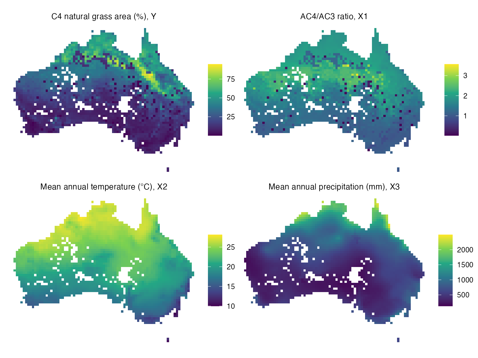
c4-data.csv: the response Y and the three predictors at 0.5°, AC4/AC3 ratio (X1), mean annual temperature (X2) and precipitation (X3). Data for 2019 from Luo et al. (2024) and the CRU-JRA climate data.The reading in one sentence: the three most spatially informative models — KNN, the neural network and XGBoost, all at E ≈ 0.50 — are not the three most accurate ones. SVR and random forest have the lowest RMSE and the highest R², yet random forest explains less spatial information than six other models — its averaged trees smooth the response surface — while KNN reaches the top E with a mid-range RMSE. The regularised linear models are last on both. Under random CV every model gains E, most of all the flexible learners that can exploit spatial proximity (GBM +17.0 %), least the linear ones (+2.1 %).
1.4 Reproduction Scope
Everything tagged Demo run regenerates from this folder with Rscript run-all.R on
R 4.6.0. The ten models' SIE and R² match reference-results.csv of the SIE repository to
machine precision (largest difference 4.4 × 10⁻¹⁶).
- The whole case study, from the raw table. Ten models are fitted under both cross-validation designs, SIE is computed for each, and the paper's figure of SIE against R² is redrawn — in about 40 seconds, with no stored predictions.
- The paper's further analyses, redrawn. The mutual information components and scale profiles, RMSE and R² under both designs, the block-vs-random comparison and the 42-setting sensitivity analysis — as figures, from the same out-of-fold predictions.
- A hand-checkable example. A 4 × 4 grid where every SIE quantity can be
computed on paper, run through the same
sie.Rfunctions.
| Item | Demo template | Published reference |
|---|---|---|
| Data | c4-data.csv (2,480 cells), as published in the SIE repository | the same table, derived from Luo et al. (2024) and CRU-JRA climate data |
| Method | sie.R from the SIE repository, unchanged | the paper's Section 2 (Eqs. 1–9) |
| Models and CV | example.R, unchanged: the paper's ten models, block and random five-fold CV, seed 42 | Section 4.2 |
| Further analyses | further-analyses.R: results/*.csv and five figures | Sections 5.1–5.2 |
| Figures | sie-vs-r2.jpg and the five figures of further-analyses.R, tagged Demo run | the paper's Figs. 5, 6, 8, 10, 11 and 14, redrawn from the published code |
| Not re-run | — | the simulation study (Figs. 1–4, Tables 1–2), the residual maps (Figs. 7, 13) and the five alternative block-to-fold assignments |
What the template generates and the published content it corresponds to.
How to use this page
- To reproduce the demo: run
Rscript run-all.R. Every figure below regenerates in under a minute. - To use SIE on your own model: §2.3 gives the data contract — a response, out-of-fold
predictions from spatial block CV, and coordinates — and §4.1 the porting steps.
sie()itself needs nothing but base R.
2 Setup, Structure & Data Contract
2.1 Environment & Dependencies
The metric is one base-R file; the packages below are only needed to fit the paper's ten models and draw the figures.
# The metric: nothing to install, sie.R uses base R only
# The case study: modelling engines and plotting helpers (from CRAN)
install.packages(c("tidymodels", "bonsai", "ranger", "xgboost", "lightgbm",
                   "kernlab", "glmnet", "kknn", "earth", "nnet",
"patchwork", "ggrepel"))| Package | Role in the pipeline | Required? |
|---|---|---|
| base R | sie(): binning, grid, mutual information, weights (sie.R); the worked example | yes |
tidymodels 1.5.0 | folds (manual_rset, vfold_cv), the recipe that standardises predictors within each training set, fit_resamples | for the case study |
ranger 0.18.0, xgboost 3.2.1.1, lightgbm 4.7.0 + bonsai 0.4.1 | random forest; XGBoost and GBM; LightGBM | for the case study |
kernlab 0.9-33, nnet 7.3-20, kknn 1.4.1 | SVR; the neural network; KNN | for the case study |
glmnet 5.0, earth 5.3.5 | elastic net and lasso; MARS | for the case study |
ggplot2, patchwork, ggrepel | the six figures | for the figures |
Package roles and the versions of the verified run, recorded in
results/session-info.txt: R 4.6.0, aarch64-apple-darwin23. With these versions the
out-of-fold predictions — and hence every figure on this page — are identical to those of the reference run. Random
forest, SVR and the neural network use random numbers; other versions or platforms can move their results
in later decimals, which example.R reports as the largest difference from the reference.
2.2 Project Structure & Configuration
One entry script runs three scripts in order. The four files from the SIE repository are used exactly as published; the tutorial adds the worked example, the further analyses and the runner.
sie/
├── run-all.R                  # entry point: steps 1-5, ~45 s
├── sie.R                      # sie(): the metric, base R      (SIE repository)
├── example.R                  # ten models, SIE, figure, check (SIE repository)
├── c4-data.csv                # 2,480 cells: lon, lat, Y, 3 predictors (SIE repository)
├── reference-results.csv      # E and R2 of the reference run  (SIE repository)
├── worked-example.R           # SIE by hand on a 4 x 4 grid
├── further-analyses.R         # further analyses: 5 figures + results/*.csv
├── figures/                   # sie-vs-r2.jpg + 5 fig-*.png    (generated)
├── results/                   # CSV tables, runtimes, session  (generated)
├── README.md
└── LICENSE # GPL-3.0There is no download step. c4-data.csv is the analysis-ready table published in the
SIE repository: the C4 natural grass area percentage and the AC4/AC3 ratio are derived from the global
C4 vegetation dataset of Luo et al. (2024), and temperature and precipitation from the CRU-JRA gridded
climate data (Harris et al. 2020; Kobayashi et al. 2015). Please cite these sources when you use the
data.
Settings
The settings sit at the top of example.R; every value is the paper's. The block grid of
the folds is set inside its fold code.
N_FOLDS <- 5                  # cross-validation folds
N_BINS  <- 20                 # equal-frequency bins for Y and residuals
SCALES  <- c(4, 6, 8, 10)     # grids of 900, 600, 450 and 360 km cells
SEED    <- 42

# Spatial block CV: a 10 x 10 block grid over the bounding box of the data
xb <- cut(S[, 1], breaks = seq(min(S[, 1]), max(S[, 1]), length.out = 11),
include.lowest = TRUE, labels = FALSE)| Parameter | Default | Origin / rationale |
|---|---|---|
N_BINS (nb) | 20 | equal-frequency bins for Y and ε; with 20 bins H(Y) ≈ log 20 nats. More bins raise the bias term |
SCALES | 4, 6, 8, 10 | grid sizes g for the mutual information, from continental (900 km) to mesoscale (360 km); the finest is set so that the bias stays at most about 0.25 of I(Y; S) |
tau | 1 | softmax temperature of the weights; fixed, which keeps the metric free of tuning (argument of sie()) |
| block grid | 10 × 10 | the CV blocks (about 360 km). Independent of SCALES: blocks set how far test data are from training data, grids set the grain at which information is measured |
N_FOLDS | 5 | five-fold block CV and five-fold random CV |
SEED | 42 | the fold assignment of both designs; the neural network uses SEED + 1 (block) and SEED + 2 (random) |
Free parameters and the published choices they follow.
2.3 Data Contract
SIE itself needs three aligned vectors: the observed response, out-of-fold predictions from a spatially separated validation, and coordinates. The case study starts one step earlier, from a table with the predictors.
Input of sie() | Type | Meaning |
|---|---|---|
y | numeric vector | the observed response |
y_hat | numeric vector, same order | out-of-fold predictions — from spatial block CV, so every prediction comes from a model that did not see its neighbourhood |
coords | two-column matrix or data frame | coordinates; the grid is laid over their bounding box, so longitude/latitude or projected units both work |
n_bins, scales, tau | numbers | bins, grid sizes and softmax temperature (defaults 20; 4, 6, 8, 10; 1) |
The schema of sie(y, y_hat, coords, n_bins = 20, scales = c(4, 6, 8, 10), tau = 1).
Missing values are not allowed.
| lon | lat | C4_grass_area_pct | AC4_AC3_ratio | MAT_celsius | MAP_mm |
|---|---|---|---|---|---|
| 142.25 | −11.25 | 39.97 | 1.981 | 26.63 | 2240.7 |
| 130.75 | −11.75 | 35.80 | 1.919 | 27.01 | 2247.0 |
The first two rows of c4-data.csv (values rounded for width): 2,480 cells of
0.5° from 113.75°E to 152.75°E and 11.25°S to 42.25°S. The response ranges from 0.03 to 94.7 %
(median 19.8 %).
- Residuals must come from spatially separated validation. Use out-of-fold predictions of spatial block CV (or another spatially separated design, such as spatial+ partitions). Residuals of a model fitted on all the data, or of random CV, let nearby observations pass spatial structure into the predictions and overstate E.
- Keep the order.
y,y_hatandcoordsmust refer to the same observations in the same order;example.Rsorts the collected predictions by row for this reason. - Give the bins room. Equal-frequency binning needs distinct quantile breaks; a response
with many tied values (for example many zeros) needs fewer bins, and
sie()stops with a message if the breaks are not unique.
3 Reproduction Pipeline, Results & Validation
3.1 Pipeline Execution
| Full run | Rscript run-all.R — ~46 s measured |
|---|---|
| Output folders | figures/ results/ |
cd sie                       # this folder
Rscript run-all.R            # full pipeline, ~45 s

Rscript worked-example.R     # step 1 alone, base R, instant
Rscript example.R # steps 2-4 alone: the script of the SIE repository| Script | What it does | Seconds |
|---|---|---|
worked-example.R | the 4 × 4 example: three models, one grid, checked against the hand values | 0.0 |
example.R | folds; ten models × block and random CV; sie() for all 20 runs; the figure; the reference check | 37.6 |
further-analyses.R | five figures (data, SIE components, accuracy, block vs random, 42-setting sensitivity) and results/*.csv | 7.8 |
| total | R 4.6.0 on an Apple-silicon laptop | 45.6 |
Measured wall-clock time, from results/runtimes.csv, written by the run itself.
Almost all of it is model fitting: ten models × two designs × five folds, the neural network five times per
fold. The further analyses reuse the stored predictions and take a few seconds.
== Step 1    worked-example.R: SIE by hand on a 4 x 4 grid ===========
Response Y (rows i = 1..4, columns j = 1..4):
     [,1] [,2] [,3] [,4]
[1,]  1.0  2.6  3.2  4.4
[2,]  1.4  2.2  3.6  4.0
[3,]  1.2  2.4  3.0  4.6
[4,]  1.6  2.0  3.4  4.2

One grid resolution (2 x 2 cells), n_bins = 2:
  model A: I(Y;S) = 0.69315  I(e;S) = 0.00000  E = 1.00000  (by hand 1.00000)
  model C: I(Y;S) = 0.69315  I(e;S) = 0.13081  E = 0.81128  (by hand 0.81128)
  model B: I(Y;S) = 0.69315  I(e;S) = 0.69315  E = 0.00000  (by hand 0.00000)
  ln 2 = 0.69315;  (3/4) ln 3 - ln 2 = 0.13081

Too fine a grid (4 x 4, one observation per cell), model A:
  I(Y;S) = 0.69315  I(e;S) = 0.69315  E = 0.00000   bias term 0.469

Worked example: all three E values equal the hand calculation.

== Step 2-4  example.R: ten models, multi-scale SIE, figure, check ===

Block CV, KNN:
Spatial information explained (SIE)
  observations: 2480 | bins: 20 | scales: 4x4, 6x6, 8x8, 10x10
  multi-scale E = 0.501
 n_grid cells I_Y_S I_e_S   E_r  bias weight
      4    15 0.670 0.258 0.615 0.054  0.199
      6    29 0.829 0.358 0.568 0.107  0.234
      8    49 0.971 0.491 0.495 0.184  0.269
     10    72 1.071 0.664 0.379 0.272  0.298

Multi-scale SIE (E) and R2 of the ten models:
  [... 20 rows: E, E_se, R2, R2_se per model and design -- drawn in figures/sie-vs-r2.jpg ...]

Figure written: figures/sie-vs-r2.jpg
Largest difference from the reference: E 4.44e-16, R2 5.55e-16 -- identical to the reference results

== Step 5    further-analyses.R: further analyses, redrawn ===========
Block CV accuracy: RMSE 8.26 (SVR) to 9.75 (Lasso); R2 0.696 (Lasso) to 0.789 (SVR)
Spearman rho of E with RMSE -0.38, with R2 0.53
Weights 900-360 km: 0.199 0.234 0.269 0.298; linear or uniform weights change E by at most 0.013
Random CV overstates E for 10 of 10 models: 2.1% to 17.0% (mean 9.9%)
Sensitivity, 42 settings: Spearman rho 0.879 to 0.988 (median 0.927)
Figures written: figures/fig-data.png, fig-sie-overview.png, fig-accuracy.png, fig-block-vs-random.png, fig-sensitivity.png

Finished in 45.6 s
3.2 Core Analytical Steps
Five steps: purpose → code → output → result → how to read it. Step 1 is the worked example;
steps 2–4 are the four parts of example.R; step 5 redraws the paper's further analyses.
SIE by hand — a 4 × 4 grid
What this step does
Before ten machine learning models, sixteen numbers. The response on a 4 × 4 grid is a
left-to-right gradient, Y(i, j) = j + o(i, j),
plus a perturbation o ∈ {0, 0.2, 0.4, 0.6} placed so that it is unrelated to
location. Three "models" are scored with two bins and a 2 × 2 grid: A learns the gradient,
C learns part of it, B is the no-model baseline. Every quantity can be checked on paper, and the script
checks the hand values against sie_scale(), the single-resolution step of sie().
Code
source("sie.R")
i <- rep(1:4, times = 4); j <- rep(1:4, each = 4)   # row, column
S <- cbind(x = j, y = i)
Y <- j + o[cbind(i, j)]                              # gradient + perturbation

Y_hat <- list(A = j,                                 # the gradient, learned
              C = Y - e_C[cbind(i, j)],              # part of it
              B = rep(0, 16))                        # nothing
for (m in names(Y_hat))
  print(sie_scale(Y, Y_hat[[m]], S, n_bins = 2, n_grid = 2))
The calculation
| i \ j | 1 | 2 | 3 | 4 |
|---|---|---|---|---|
| 1 | 1.0 | 2.6 | 3.2 | 4.4 |
| 2 | 1.4 | 2.2 | 3.6 | 4.0 |
| 3 | 1.2 | 2.4 | 3.0 | 4.6 |
| 4 | 1.6 | 2.0 | 3.4 | 4.2 |
The response Y (rows i, columns j). The median is 2.8, so the two equal-frequency bins are exactly columns 1–2 (low) and columns 3–4 (high): the spatial structure of Y.
The response. Each 2 × 2 cell lies entirely in one half of the grid, so every cell is pure in Y's bin: H(Y | S) = 0 and I(Y; S) = H(Y) = ln 2 = 0.69315 nats.
Model A leaves the perturbation, {0, 0.2, 0.4, 0.6}; every cell holds two low and two high residuals, exactly the overall shares, so I(ε; S) = 0 and E = 1. Model B predicts nothing, so ε = Y, I(ε; S) = ln 2 and E = 0. Model C leaves a 3 : 1 imbalance of low and high residuals in every cell; with p(y) = ½ and p(s) = ¼, Eq. (4) gives
Example output
Response Y (rows i = 1..4, columns j = 1..4):
     [,1] [,2] [,3] [,4]
[1,]  1.0  2.6  3.2  4.4
[2,]  1.4  2.2  3.6  4.0
[3,]  1.2  2.4  3.0  4.6
[4,]  1.6  2.0  3.4  4.2

One grid resolution (2 x 2 cells), n_bins = 2:
  model A: I(Y;S) = 0.69315  I(e;S) = 0.00000  E = 1.00000  (by hand 1.00000)
  model C: I(Y;S) = 0.69315  I(e;S) = 0.13081  E = 0.81128  (by hand 0.81128)
  model B: I(Y;S) = 0.69315  I(e;S) = 0.69315  E = 0.00000  (by hand 0.00000)
  ln 2 = 0.69315;  (3/4) ln 3 - ln 2 = 0.13081

Too fine a grid (4 x 4, one observation per cell), model A:
  I(Y;S) = 0.69315  I(e;S) = 0.69315  E = 0.00000   bias term 0.469

Worked example: all three E values equal the hand calculation.- The ordering is the point. A > C > B: the more of the gradient a model learns, the less its residuals depend on location. Model C's 3:1 imbalance is exactly the kind of leftover structure that RMSE averages away.
- E = 0 for the baseline is an identity, not a coincidence: with Ŷ = 0 the residuals are the response, so the ratio is one.
- Too fine a grid destroys the measurement. With 4 × 4 cells every cell holds one observation and is trivially pure, so I(Y; S) = I(ε; S) = ln 2 for any model and E collapses to 0; the bias term (0.469) is then 68 % of I(Y; S). This is why the finest grid of the case study is chosen with the bias rule.
- Real data never reach 1. This table is an exact population; a sample estimate of I(ε; S) for pure noise is positive, which is why the paper's simulation tops out at 0.802.
Ten models under block and random cross-validation
What this step does
Builds the two fold designs and collects out-of-fold predictions of the ten models for all 2,480 cells.
For block CV, a 10 × 10 grid over the bounding box gives 72 occupied blocks of about 360 km,
assigned at random to five folds (14 or 15 blocks, 433–592 cells per fold). Random CV draws five folds of
496 cells. Nine models run through one tidymodels workflow with predictors standardised inside each
training set; the neural network is fitted directly with nnet and averaged over five random
initialisations per fold, to keep spatially unstructured fitting noise out of the residuals.
Code
block_id <- as.integer(interaction(xb, yb, drop = TRUE))   # 72 occupied blocks
fold_of_block <- sample(rep(seq_len(N_FOLDS),
                            length.out = length(unique(block_id))))
fold_block <- fold_of_block[block_id]                      # fold of every cell

rec <- recipe(C4_grass_area_pct ~ ., data = df_model) |>
  step_normalize(all_predictors())
models <- list(
  random_forest = rand_forest(trees = 500) |> set_engine("ranger") |> set_mode("regression"),
  xgboost = boost_tree(trees = 500, learn_rate = 0.1, tree_depth = 3) |>
    set_engine("xgboost") |> set_mode("regression"),
  knn = nearest_neighbor(neighbors = 10) |> set_engine("kknn") |> set_mode("regression")
  # ... lightgbm, svr, elastic_net, lasso, gbm, mars: see example.R
)
oof_block  <- oof_cv(folds_block,  "block")    # fit_resamples(), predictions by row
oof_random <- oof_cv(folds_random, "random")
oof_block$neural_net <- oof_nn(fold_block, "block", SEED + 1)   # 64 units, 5 starts
The ten models
| Class | Models and fixed settings | Learning principle |
|---|---|---|
| Tree ensembles | random forest (500 trees); XGBoost (500 trees, rate 0.1, depth 3); GBM (500, 0.05, depth 3); LightGBM (500, 0.05, 15 leaves) | piecewise-constant surfaces from recursive partitioning; averaging (bagging) or sequential correction (boosting) |
| Smooth nonlinear | SVR (radial kernel); neural network (64 hidden units, 100 epochs, mean of 5 starts) | global smooth nonlinear functions |
| Instance-based | KNN (k = 10) | local averaging of the nearest observations in feature space |
| Linear and splines | elastic net (penalty 0.1, mixture 0.5); lasso (0.1, 1.0); MARS | global linear hypotheses with shrinkage, extended by piecewise-linear bases (MARS) |
The paper's Table 3, with the settings of example.R. Hyperparameters are
fixed at regularised values rather than tuned, because overfitted or unstable fits would add spatially
unstructured noise to the residuals and distort a residual-based metric.
The blocks and the mutual-information grids are separate settings that happen to share a size at the finest scale: the 10 × 10 blocks decide how far each test cell is from the training data; the 4–10 grids of Step 3 decide the grain at which spatial information is measured. Everything downstream — SIE, RMSE and R² — is computed from the same out-of-fold vectors, so the metrics are compared on identical validation partitions.
Multi-scale SIE of every model
What this step does
Applies sie() to the out-of-fold predictions of each model under each design, with 20 bins
and the four grids. E is computed from all 2,480 residuals together; its standard error comes from
the E values computed within each of the five folds. R² is computed within each held-out fold and
averaged. The full output of sie() is printed for KNN, the top model.
Code
E <- sie(Y, oof_block$knn, S, n_bins = N_BINS, scales = SCALES)
E$E          # multi-scale SIE
E$profile    # one row per grid: cells, I_Y_S, I_e_S, E_r, bias, weight

# all models, both designs: E, its fold SE, R2 (fold mean) and its SE
res <- rbind(evaluate(oof_block,  fold_block,  "block"),
             evaluate(oof_random, fold_random, "random"))
Example output
Block CV, KNN:
Spatial information explained (SIE)
  observations: 2480 | bins: 20 | scales: 4x4, 6x6, 8x8, 10x10
  multi-scale E = 0.501
 n_grid cells I_Y_S I_e_S   E_r  bias weight
      4    15 0.670 0.258 0.615 0.054  0.199
      6    29 0.829 0.358 0.568 0.107  0.234
      8    49 0.971 0.491 0.495 0.184  0.269
     10    72 1.071 0.664 0.379 0.272  0.298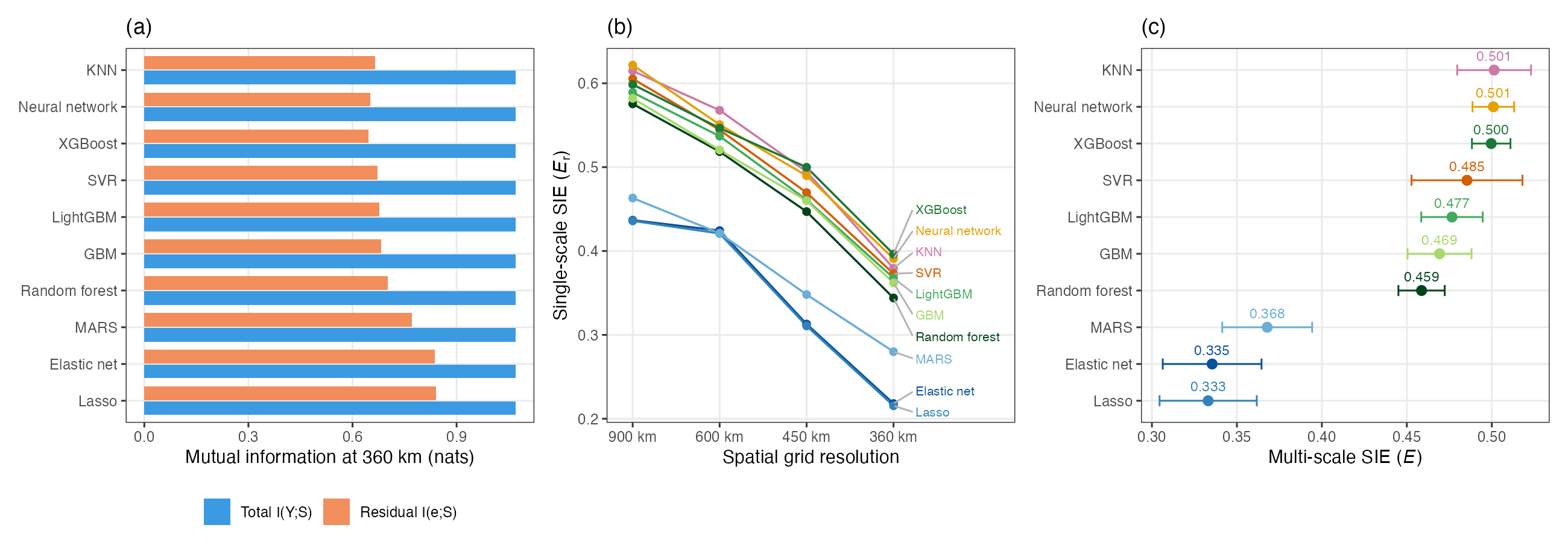
- Read the profile row by row. At 900 km the response has 0.670 nats of spatial information and KNN leaves 0.258 of it, Er = 0.615. At 360 km there is more to explain (1.071 nats) and more is left (0.664), Er = 0.379: fine-grained dependence is harder to absorb, and Er falls with resolution for all ten models.
- The weights are nearly flat (0.199–0.298) and identical for every model, because they come from Y alone. Spatial information is spread across the four scales rather than concentrated at one, so the aggregate is insensitive to the weighting rule: linear or uniform weights change E by less than 0.013 and leave the ranking unchanged (printed by Step 5).
- The bias column is the guard rail. At 360 km it is 0.272 nats, about a quarter of I(Y; S) — the paper's limit for the finest grid. At 1.071 / log 20, location accounts for about 36 % of the entropy of C4 grass cover at this grain.
SIE against R², and the check against the reference
What this step does
Draws E against R² for both designs (the featured figure at the top of this page) and compares
the run with reference-results.csv, the results of the same script on the machine used for
the paper. On the verified setup the largest differences are 4.4 × 10⁻¹⁶ in E and
5.6 × 10⁻¹⁶ in R²: identical.
R² in this tutorial
R² is computed as 1 − SSE/SST within each held-out fold and averaged over the five folds, with the fold-to-fold standard error as error bar (the paper's Eq. 11). E is computed from all out-of-fold residuals together and its standard error from the five within-fold values. Step 5 adds RMSE on the same folds.
- Two axes, two questions. Up is "how close are the predictions"; right is "how much of the geography have they captured". SVR is highest; KNN, the neural network and XGBoost are furthest right. The neural network and SVR, the smooth nonlinear class, combine both best.
- High accuracy with low E means the predictors carry limited spatial information and the model fits well on average while leaving structured residuals; high E with low accuracy would point to unstructured noise in the predictions. Read E together with an accuracy metric from the same validation.
- The right panel moves everything up and right. Random CV inflates both accuracy and E — the same proximity leak, seen in two metrics (Step 5).
The paper's further analyses, redrawn
What this step does
Takes the out-of-fold predictions that example.R left in the session and redraws the
paper's further analyses without refitting anything: the data maps, the mutual information components and
scale profiles of Step 3, RMSE and R² under both designs, the block-vs-random comparison of E, and
the sensitivity of E to the discretization over 6 bin counts × 7 grids. Tables of every quantity go to
results/; the console prints a short summary.
Code
# RMSE and R2 = 1 - SSE/SST within each held-out fold, both designs
acc <- rbind(fold_stat(oof_block,  fold_block,  rmse, "Block CV"),
             fold_stat(oof_block,  fold_block,  r2,   "Block CV"),
             fold_stat(oof_random, fold_random, r2,   "Random CV"))

# 42 settings from the same block CV residuals: no refitting
NB <- c(5, 10, 15, 20, 25, 30)
NG <- c(4, 6, 8, 10, 12, 16, 20)                  # 900 ... 180 km
single <- sie_scale(Y, oof_block[[m]], S, n_bins = nb, n_grid = ng)  # per model, nb, ng
rho <- cor(e, ref_rank, method = "spearman")      # vs multi-scale E at n_b = 20
Example output
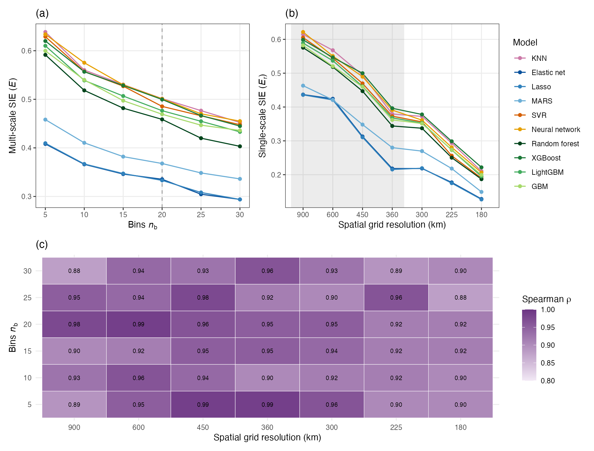
- Magnitude moves, order holds. Refining either the bins or the grid lowers E for every model — mean Er falls from 0.552 at 900 km to 0.181 at 180 km — because the bias term grows (0.05 to 0.95 nats) faster than I(Y; S) (0.67 to 1.58). The ranking barely changes: the leading group stays on top in 40 of 42 settings, the linear models stay last in all of them. Compare E across models only at identical settings and sample sizes.
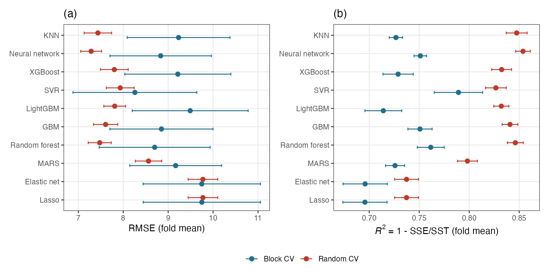
- Random CV is optimistic in both metrics, for the same reason. Mean E rises from 0.443 to 0.489, mean RMSE falls from 9.12 to 8.15 and mean R² rises from 0.734 to 0.815. Randomly held-out cells have training neighbours that reproduce local structure the predictors cannot, so residuals look less spatial. The flexible learners profit most (GBM +17.0 %, LightGBM +14.9 %), the linear models least (+2.1 %).
- Accuracy ranks the models differently. SVR has the lowest RMSE (8.26) and the highest R² (0.789), random forest the second-lowest RMSE, while the leading E group — KNN, the neural network and XGBoost — sits mid-range in accuracy. Across the ten models Spearman ρ is −0.38 between E and RMSE and 0.53 between E and R².
- Multi-scale is not single-scale. At 360 km alone the mean Er is 0.333, at the coarsest grid well above E; the aggregate integrates the grains instead of depending on one.
3.3 Reading the Results Together
- SIE separates models. E runs from 0.333 (lasso) to 0.501 (KNN): the instance-based, smooth nonlinear and tree-ensemble models between 0.459 and 0.501, the linear and spline models between 0.333 and 0.368.
- It is not accuracy in disguise. Spearman ρ = −0.38 with RMSE and 0.53 with R²; random forest is second in RMSE and seventh in E.
- Block CV keeps it honest. Random CV overstates E for all ten models, by 2.1–17.0 % (mean 9.9 %), most for the models that exploit spatial proximity.
- The ranking is robust to the weighting rule (linear or uniform weights change E by less than 0.013) and to 42 discretization settings (ρ ≥ 0.879).
- Mechanism. Mutual information compares the distribution of residuals inside each grid cell with their overall distribution. Any systematic difference — a regional bias, a gradient, a zone of larger errors — registers, including nonlinear forms that an average error or a correlation-based statistic such as Moran's I can miss.
- What a high E buys. Higher E with equal or better accuracy means the model has learned more of the geography of the response. Spatially unstructured noise can also weaken the residuals' dependence on location while worsening accuracy, so E is read together with RMSE or R² from the same validation, never alone.
- What the weights say. The near-flat softmax profile (0.199–0.298) says that spatial information in C4 grass cover is spread over continental to mesoscale grains; a strongly peaked profile would point to one dominant scale.
1) the last line of example.R — identical to the reference, or the size of the difference.
2) the sie() profile of your best model — is the bias at the finest grid still small relative
to I(Y; S)? 3) figures/fig-sie-overview.png — how much spatial information each
model leaves, scale by scale. 4) figures/sie-vs-r2.jpg — where each model sits on the two axes.
5) figures/fig-block-vs-random.png — how much of each model's E came from proximity.
4 Adaptation, Writing & Reproducibility
4.1 Port to Your Domain
SIE applies to any spatial prediction with a continuous response — soil properties, air quality, vegetation cover, land surface temperature, urban indicators — and to any model, from kriging to a deep network: it only reads predictions. The port is one function call after your own block cross-validation:
source("sie.R")                       # base R, no packages

# y_hat: out-of-fold predictions of YOUR model from spatial block CV,
# in the same row order as y and coords
E <- sie(y = mydata$y, y_hat = y_hat,
         coords = mydata[, c("x", "y")],
         n_bins = 20, scales = c(4, 6, 8, 10))
E$E                                    # multi-scale SIE
E$profile                              # check: bias small relative to I_Y_S
max(E$profile$bias / E$profile$I_Y_S)  # the case study stays at about 0.25
What to edit
- The folds. Build spatial blocks for your study area and keep every model on the same folds. The case study's 10 × 10 block grid over the bounding box is a simple default; blocks larger than the range of spatial dependence of the residuals give a stricter test.
- The models. Collect the out-of-fold predictions of each model you compare, aligned with the data rows. Fix or nest-tune hyperparameters inside the training folds; avoid settings that make the fits unstable, since unstructured noise also changes E.
n_bins. 20 suits a few thousand observations. Fewer observations or many tied values call for fewer bins.scales. From a coarse grid with a handful of occupied cells to the finest grid at which the bias term stays small relative to I(Y; S). Fix them before looking at the models, and do not choose the scale that makes a favoured model look best.- Nothing else:
taustays at 1.
Choosing grids and bins with the bias rule
- Compute the profile of the response first.
sie(y, y_hat = rep(0, length(y)), coords)returns I(Y; S), occupied cells and the bias term for every candidate grid without any model; drop grids whose bias exceeds about a quarter of I(Y; S). - Mind the occupied cells. Irregular study areas leave many grid cells empty — 72 of 100 in the Australian case — and only occupied cells count in the bias term.
- Same settings for every model. E values are comparable only under identical bins, grids and sample size; report them with those settings.
Report the validation design (block size or grid, number of folds, seed), nb, the grid sizes and their cell sizes, the softmax weights, the multi-scale E with its fold standard error, the scale profile of at least the leading models, and an accuracy metric computed from the same out-of-fold predictions. If you also report random CV, show both designs side by side.
4.2 Write the Paper
The published study separates the metric from its evidence: define spatial information and SIE, check the metric where the answer is known, then use it to compare real models along a dimension accuracy does not cover.
| Manuscript section | Template output | Writing job |
|---|---|---|
| Methods | sie.R, §1.2 | spatial information as I(Y; S), the residuals from block CV, the discretization and bias term, the softmax weights; state that the weights depend on Y only |
| Data and models | c4-data.csv, example.R | the response, predictors and sources; the models and fixed settings; both CV designs |
| Results — SIE | the sie() profile, results/scale-profile-block.csv | mutual information components, scale profiles and multi-scale E per model |
| Main figure | figures/sie-vs-r2.jpg, results/accuracy.csv | accuracy against E; the rank correlations; which models lead on which axis |
| Results — robustness | results/sensitivity-*.csv, the sensitivity figure | magnitude vs ranking across bins and grids; the bias rule for the finest grid |
| Results — CV design | results/block-vs-random.csv | the overstatement under random CV, per model and on average |
| Discussion | §3.3 | why mutual information sees what error metrics average away; where SIE sits among validation metrics |
Where each manuscript element draws its material from.
Manuscript skeleton
1  Introduction        - spatial validation relies on error metrics; no measure
                          of how much spatial structure a model explains, and none
                          designed for block cross-validation (aims)
2  SIE metric          - 2.1 spatial information I(Y;S)
                          2.2 E = 1 - I(e;S)/I(Y;S); discretization and bias
                          2.3 residuals from spatial block CV
                          2.4 multi-scale SIE with softmax weights
3  Simulation          - controlled learning ladder; boundary cases; robustness
4  Case study          - data; ten models; block and random CV; SIE settings
5  Results             - SIE per model; SIE vs accuracy; single vs multi-scale;
                          sensitivity; block vs random CV
6  Discussion          - what mutual information captures; joint reading with
                          accuracy; position among validation metrics; limits
7  Conclusions         - 6-8 sentences answering the aims
4.3 Final Reproducibility Package
| Code | sie.R + example.R (SIE repository) + worked-example.R + further-analyses.R + run-all.R |
|---|---|
| Data | c4-data.csv and reference-results.csv (SIE repository) |
| Results | results/*.csv + figures/ + results/runtimes.csv and results/session-info.txt |
What is in the download, and what is not
Included in sie-code-and-data.zip | Not included |
|---|---|
the five R scripts, c4-data.csv, reference-results.csv, every CSV in
results/ with the runtimes and session record, the six figures in
figures/, README.md and LICENSE |
the out-of-fold predictions, which the run recomputes in under a minute; the simulation study, whose results are reported in the paper |
The four files from the SIE repository are byte-identical to
github.com/yongzesong/SIE; the repository remains the
authoritative source of sie().
- Delete
results/andfigures/, runRscript run-all.R— the last line of step 4 reports "identical to the reference results" and step 5 writes the five figures. - The bins, grids, fold design and seed you report match the settings at the top of
example.R. - Package versions are named: random forest, SVR and the neural network depend on them.
- E is reported with its fold standard error, next to an accuracy metric from the same folds.
results/session-info.txtis included in the deposit.
Isn't this just residual autocorrelation? → Moran's I tests whether neighbouring residuals are alike; SIE measures how much of the response's total dependence on location is gone, and mutual information also registers changes in spread or shape across space. Doesn't the result depend on the bins and grid? → the magnitude does, which is why settings are fixed and reported; the ranking does not (ρ ≥ 0.879 over 42 settings). Why multi-scale? → the weights come from Y alone, so no scale is chosen after seeing the models, and the near-flat weights show that information is spread across scales. Why not random CV? → it overstates E for every model, by up to 17 %, through the same proximity leak that inflates its accuracy.
References & credits
Every figure on this page was generated by the scripts in this folder from the code and data of the SIE repository.
- Song Y (2026). Spatial information explained by prediction models under block cross-validation. ISPRS Journal of Photogrammetry and Remote Sensing 242:984–1000. doi:10.1016/j.isprsjprs.2026.09.034 (source of the method)
- SIE code, data and example —
github.com/yongzesong/SIE
(
sie.R,example.R,c4-data.csvand the reference results, as published with the paper) - Luo X, Zhou H, Satriawan TW, Tian J, Zhao R, Keenan TF, Griffith DM, Sitch S, Smith NG, Still CJ (2024). Mapping the global distribution of C4 vegetation using observations and optimality theory. Nature Communications 15:1219. doi:10.1038/s41467-024-45606-3 (C4 grass area and the AC4/AC3 ratio)
- Harris I, Osborn TJ, Jones P, Lister D (2020). Version 4 of the CRU TS monthly high-resolution gridded multivariate climate dataset. Scientific Data 7:109. doi:10.1038/s41597-020-0453-3; Kobayashi S, et al. (2015). The JRA-55 reanalysis. Journal of the Meteorological Society of Japan 93:5–48. doi:10.2151/jmsj.2015-001 (temperature and precipitation)
- The SIE method article — yongzesong.com/sie/ (definition, properties, evaluation and related methods)