Reproducible models · Tutorial 9 of 13
Reproducing the Spatial Delta Model for Accessibility
A complete walkthrough of the Spatial Delta Model — which separates how much greenspace is there from how easily it can actually be reached and used, and studies the gap between them — from raw data to manuscript, on the published Perth case.
To cite the SDM model and its R packages and codes in publications, please use:
Lin G, Song Y, Xu D, Swapan MSH, Wu P, Hou W, Xiao Z (2024). Interpreting differences in access and accessibility to urban greenspace through geospatial analysis. Int J Appl Earth Obs Geoinf 129:103823. doi · PDF
Song Y, Wang J, Ge Y, Xu C (2020). An optimal parameters-based geographical detector model. GIScience & Remote Sensing 57(5):593–610. doi · OPGD tutorial
R/ pipeline scripts · config/project-config.R · data/ (8,259 residential blocks with access, accessibility and their difference at six walking times; 9,449 block polygons) · tests/ · run-all.R — unzip and run Rscript run-all.R test from the SDM/ folder root.
1 Method Overview & Reproduction Scope
1.1 Core Idea
Two neighbourhoods can have the same amount of parkland nearby and be entirely different places to live. In one the park is across the road, uncrowded, easy to walk to. In the other the same hectares sit behind a motorway, shared with ten thousand people. Counting the greenspace cannot tell them apart.
The Spatial Delta Model takes that seriously by measuring both quantities and studying their difference. Access (α) is how much greenspace is reachable within a walking time — a count of supply. Accessibility (β) is how easy it is to actually reach and use, computed with a floating catchment model that discounts supply by travel distance and shares it among everyone competing for it. Both are standardised, and the model's subject is
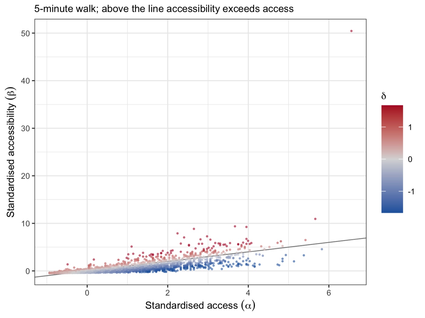
The sign is a diagnosis. Where δ > 0 the greenspace that exists is easy to reach and lightly shared — the environment is doing more than its raw endowment suggests. Where δ < 0 the greenspace is there on paper but hard to use. Neither is visible from α or β alone.
- Research problem: access and accessibility are routinely treated as the same thing, so places where supply exists but cannot be used look identical to places where it can.
- One-line contribution: SDM standardises both measures onto a common scale, subtracts them, and turns the residual into a mapped, classifiable, explainable quantity.
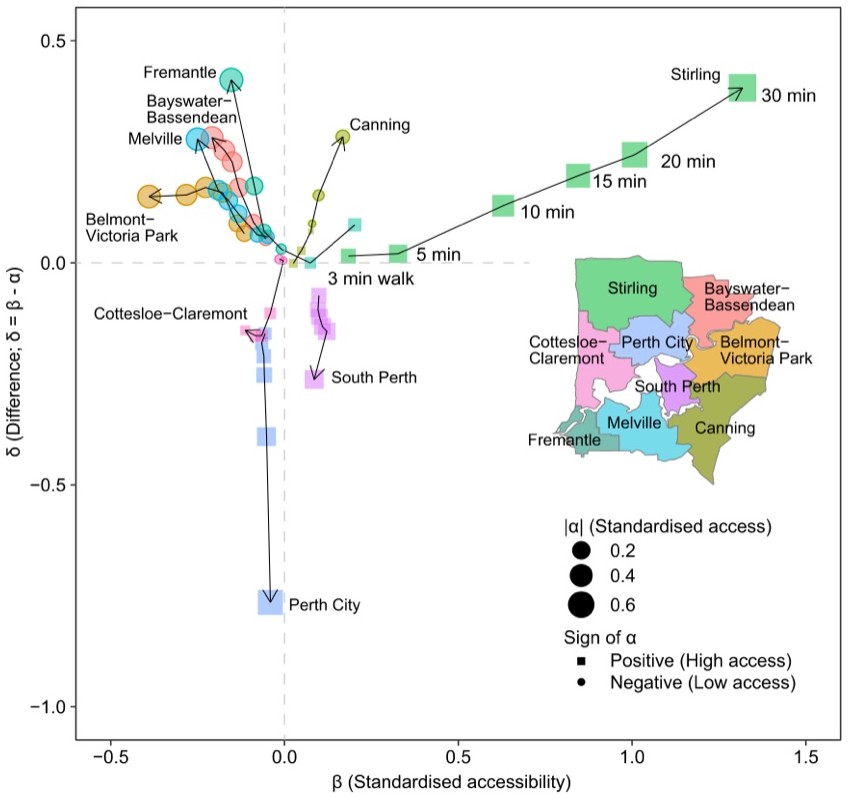
- Why it matters: the gap is not noise. In the demo below it is spatially organised, it reverses with the walking distance considered, and roughly a quarter of it is explained by measurable features of the urban fabric.
Count the greenspace within a walk (α) → measure how easily it can really be reached and used (β) → put both on the same scale and subtract → map, classify and explain the difference. Everything on this page serves that line.
R 4.1+ with sf, rpart, GD and ggplot2.
The Perth case data ship in this folder. The full pipeline takes about 15 seconds. One
optional extra, catchment, is needed only for the demonstration in
Step 2 that recomputes accessibility from the geometry.
1.2 Method Logic
SDM runs in four movements: measure the two quantities, difference them, classify the result, and explain it.
Key concepts and equations
- Access (α) — the total greenspace area within the walking distance d₀:
αi = Σj : dij ≤ d₀ GjSupply, and nothing else. Two blocks with the same total score the same however that supply is arranged or however many people share it.
- Accessibility (β) — a Modified Gaussian Two-Step Floating Catchment Area:
βi = Σj : dij ≤ d₀ Gj f(dij)² / Σk : djk ≤ d₀ Pk f(dkj)Each greenspace is discounted by how far away it is and divided among the population that can also reach it, so crowding and effort both enter. The decay f is Gaussian and truncated at d₀.
- The difference (δ) — both standardised, then subtracted. Standardising is what makes the subtraction meaningful: α is an area and β is a ratio, so they are only comparable once each is expressed in standard deviations of its own distribution.
- Spatial scale — everything is computed at six walking times (3–30 minutes, at 5 km/h), because "within reach" is a choice, not a fact, and the answer changes with it.
- Explaining δ — each candidate variable is cut into spatial strata by a regression tree, and the geographical detector scores how much of δ those strata account for (the Power of Determinant). Every variable appears twice: as its own value, and in a contextualised form carrying its local spatial pattern, so the analysis can say whether what matters is the quantity at a place or its arrangement around it. The detector is the same machinery as the OPGD tutorial.
1.3 Reproduction Scope
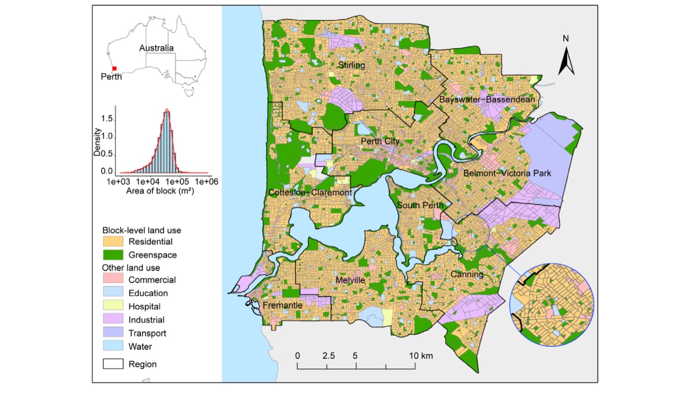
Everything tagged Demo run regenerates from this folder; everything tagged Published reference is a static image from the article. It runs end to end with R 4.6.0.
The α and β values used from Step 3 onward are the authors' own, shipped in
data/mbvars.csv, so the delta, the classification and the driver analysis are
the published ones. Step 2 demonstrates how those two measures are produced by
recomputing them from the block geometry — but with straight-line distances, whereas the
published β used road-network distances built in QGIS. The demonstration therefore matches
the practical tutorial's printed figures, not the published columns; §3.2 gives the
correlations and §2.4 explains the network step.
| Item | Demo template | Published reference |
|---|---|---|
| Data | 8,259 residential mesh blocks with α, β and δ at six walking times, and 9,449
block polygons (data/) |
the same Perth greenspace case |
| Method | catchment for the MG2SFCA demonstration; rpart +
GD for the driver analysis |
Lin et al. (2024) §3, and the accompanying tutorial |
| Tables | results/delta-summary.csv, green-city-classification.csv,
drivers-pd.csv, interaction-pid.csv |
paper Figs 5–7 and its interaction table |
| Figures | fig01–fig06 from R/p01–p03 |
paper Figs 1, 3, 4, 5, 6, 7 embedded as reference images |
What the template regenerates versus what is shown as published reference.
How to use this page
- To reproduce the demo:
Rscript run-all.R test, thenRscript run-all.R. - To apply SDM to your own city: §2.3 gives the data contract, §2.4 the network-distance step, and §4.1 the porting checklist.
- To understand the detector: the driver analysis in Step 4 uses the same machinery as the OPGD tutorial, which covers it in depth.
2 Setup, Structure & Data Contract
2.1 Environment & Dependencies
Four packages carry the pipeline. A fifth is needed only for the Step 2 demonstration, and the step reports and continues without it.
# The pipeline
install.packages(c("sf", "rpart", "GD", "ggplot2"))

# Only for the accessibility demonstration in Step 2. This one lives on GitHub.
install.packages("remotes")
remotes::install_github("uva-bi-sdad/catchment")| Package | Role in the pipeline | Required? |
|---|---|---|
sf | block geometry, centroids, distances, the maps | yes |
rpart | regression trees that cut each variable into spatial strata | Steps 4–5 |
GD | the geographical detector: Power of Determinant and interactions | Steps 4–5 |
ggplot2 | the six figures | figures only |
catchment | catchment_ratio() — the MG2SFCA demonstration | Step 2 only |
Package roles. The environment is in env/session-info.txt.
2.2 Project Structure & Configuration
SDM/
├── sdm.html                        # this guide
├── run-all.R                       # entry point: full run, single steps, figures, test
├── assets/                         # figures shown in this guide (web copies)
├── config/project-config.R         # the ONLY file to edit for a new city
├── R/
│   ├── 00-config.R, 01-helpers.R   # paths, IO, column conventions
│   ├── 10-prepare-data.R           # read the table and the geometry, check the identity
│   ├── 20-access-accessibility.R   # how alpha and beta are produced (demonstration)
│   ├── 30-delta.R                  # delta, the green-city classification, by region
│   ├── 40-drivers-gozh.R           # Power of Determinant at every walking time
│   ├── 50-interactions.R           # pairwise interaction detector
│   ├── 90-tables.R                 # LaTeX tables + session info
│   └── p01 … p03                   # figure scripts
├── data/
│   ├── mbvars.csv                  # 8,259 blocks: alpha, beta, delta + 12 variables
│   ├── blocks.gpkg                 # 9,449 polygons: 8,276 residential, 1,173 parkland
│   ├── regions.gpkg                # the nine SA3 regions
│   └── provenance.md               # where every file came from
├── tests/                          # test-01 the published table; test-02 model properties
├── env/                            # requirements.md, session-info.txt
├── results/  tables/  figs/        # generated output, never hand-edited
Main configuration file
ANALYSIS_FILE <- "data/mbvars.csv"   # alpha, beta, delta + explanatory variables
BLOCKS_FILE   <- "data/blocks.gpkg"  # consumers and providers, as polygons
ID_COL        <- "MB_CODE21"         # joins the table to the geometry
REGION_COL    <- "SA3"

# "Within reach" is a choice, so the model is evaluated at six of them.
WALK_TIMES     <- c(3, 5, 10, 15, 20, 30)            # minutes
WALK_DISTANCES <- c(250, 417, 833, 1250, 1667, 2500) # metres, at 5 km/h

ACCESS_PREFIX        <- "u"    # alpha
ACCESSIBILITY_PREFIX <- "v"    # beta
DELTA_PREFIX         <- "df"   # delta = beta - alpha

# Six variables, each also in a contextualised form carrying its local pattern
VARS_RAW <- c("popdenskm2","dwedenskm2","shapefacto",
              "compactrat","neargsdist","neargsarea")
VARS_CTX <- c("lisav1","lisav2","lisav3","lisav4","lisav5","lisav6")

TREE_MINBUCKET <- 10 # smallest terminal node a stratifying tree may create| Parameter | Default | Origin / rationale |
|---|---|---|
WALK_TIMES | 3–30 min | the paper's Table 2; distances follow from 5 km/h, the standard pedestrian speed |
TREE_MINBUCKET | 10 | the authors' value: strata smaller than ten blocks would score highly by chance |
DEMO_TIME | 3 min | the walking time the practical tutorial works through, so the demonstration can be checked against it |
INTERACTION_TIME | 5 min | a short walk, where the difference is most spatially organised |
Free parameters and the published choices they follow.
2.3 Data Contract
SDM needs two things: a table with the two measures at each spatial scale, and the geometry those measures were computed on.
| File | Columns | Meaning |
|---|---|---|
ANALYSIS_FILE | MB_CODE21, SA3 | block identifier and region |
u3 … u30 | standardised access (α) at each walking time | |
v3 … v30 | standardised accessibility (β) | |
df3 … df30 | the difference (δ), and the model's subject | |
BLOCKS_FILE | MB_CATEGOR | which blocks are consumers (residential) and which are providers (parkland) |
Person, AREASQKM21 | demand and supply |
Required schema. Column names and prefixes are declared in the config, not hard-coded.
MB_CODE21 is an eleven-digit code. Read as a number it loses precision —
50021000000 becomes 5.0021e+10 — and silently stops matching the
geometry for a subset of blocks. The pipeline forces it to character on read, and
tests/test-01 checks that all 8,259 rows still find their polygon. It is worth
checking on your own data: the failure is quiet and costs you rows, not an error.
2.4 Network Distances: the Manual Step
One part of the published workflow is not in the pipeline, and cannot be: the distances behind the published β are measured along the road network, not in straight lines, and the network was built by hand in QGIS. It matters — a park two hundred metres away across a river is not two hundred metres away — and it is why the demonstration in Step 2 does not reproduce the published columns.
The accompanying tutorial documents the procedure. In outline:
- Get the road network. In QGIS, install the QuickOSM plugin (Plugins → Manage and Install Plugins), query OpenStreetMap for the highway layer over the study area, and export it as a shapefile.
- Build the origins and destinations. Residential block centroids are the origins, greenspace centroids the destinations.
- Run the network analysis. QGIS's routing tool takes the road layer, the origins and the destinations, and returns a matrix of shortest-path distances along the network.
- Bring it back into R. Export the result and pass it to
catchment_ratio()as thecostargument, in place of the straight-line distances the function computes by default.
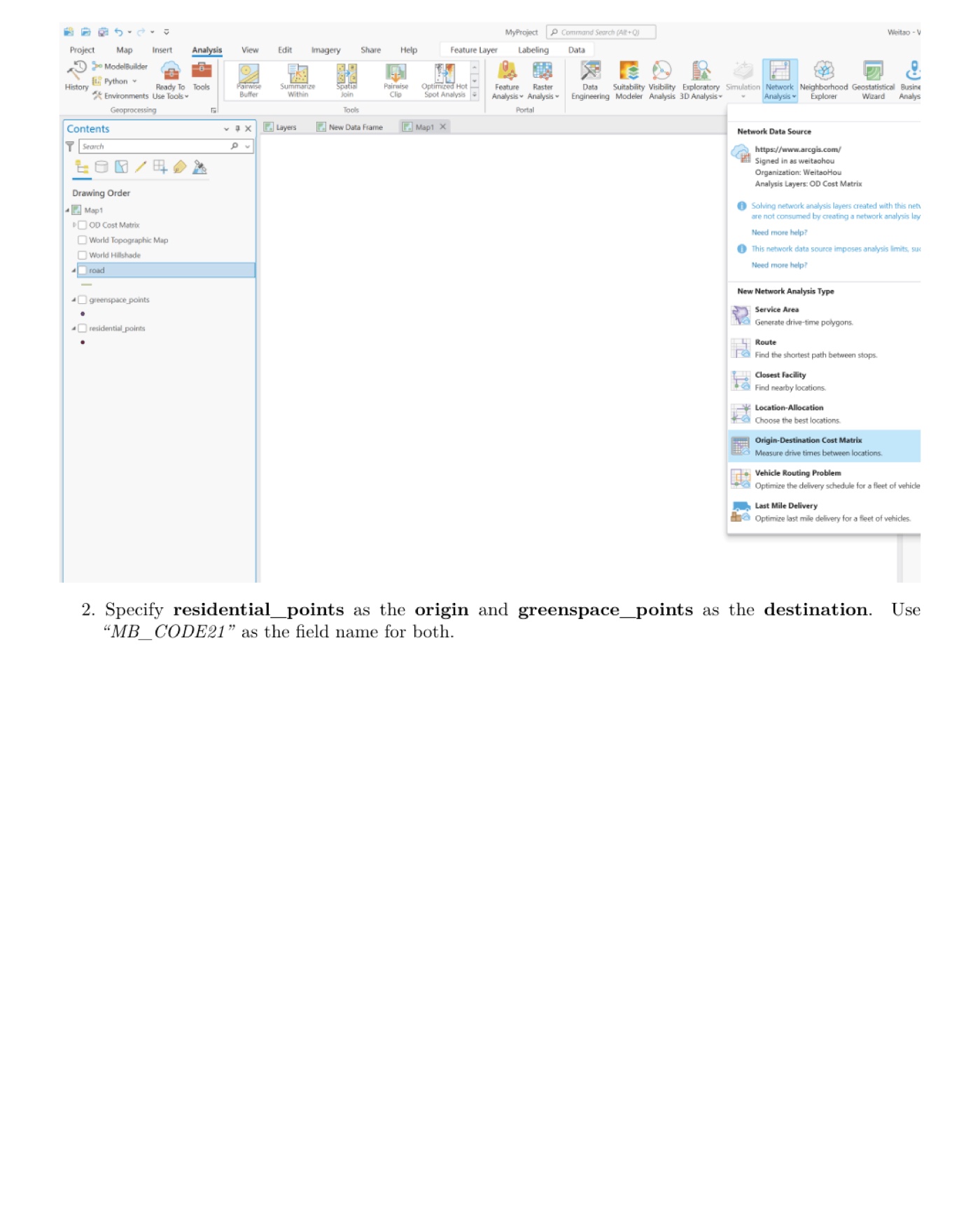
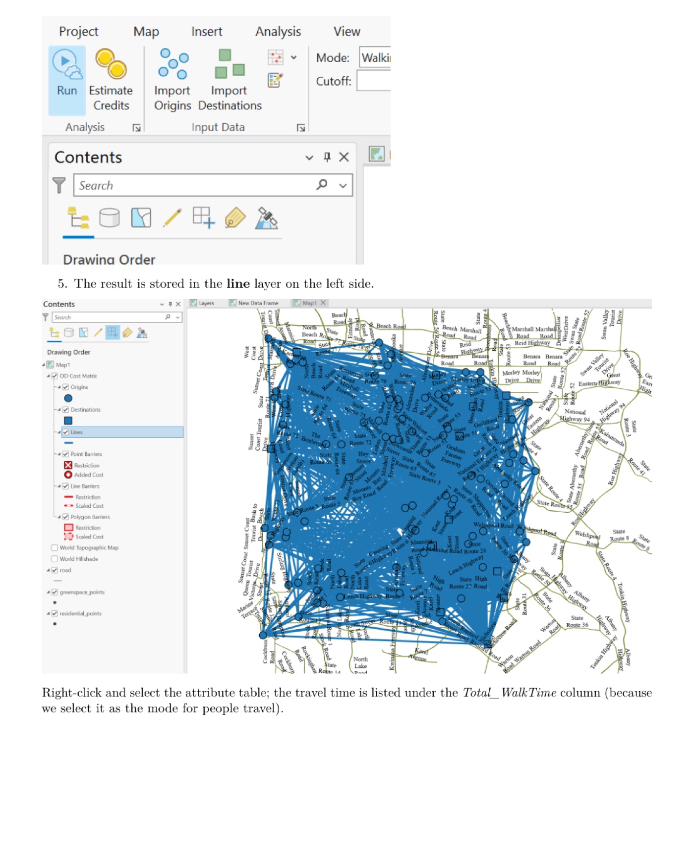
Straight-line distance flatters accessibility everywhere that movement is obstructed — rivers, railways, motorways, cul-de-sacs — and those obstructions are exactly what distinguishes access from accessibility. If you can only manage Euclidean distances, say so plainly: the δ you compute will understate the gap in precisely the places the model exists to find. One practical middle path is to run both and report the difference as a sensitivity analysis.
3 Reproduction Pipeline, Results & Validation
3.1 Pipeline Execution
| Full run | Rscript run-all.R (~15 s) |
|---|---|
| Verification | Rscript run-all.R test — do this first |
| Output folders | results/ tables/ figs/ data/derived/ |
cd SDM                     # this folder
Rscript run-all.R test     # 1. check the published table is intact
Rscript run-all.R          # 2. full pipeline

Rscript run-all.R 30 40    # re-run single steps (10 20 30 40 50 90)
Rscript run-all.R figures # only the figure scriptsProject : sdm-demo
Domain : urban greenspace, Perth
== Step 1/5 Prepare data ======================================
analysis table: 8259 residential blocks, 47 columns
regions: 9 (Bayswater-Bassendean, Belmont-Victoria Park, Canning ...)
scales: 3/5/10/15/20/30 minutes (250/417/833/1250/1667/2500 m) at 5 km/h
delta = accessibility - access holds to 1.0e-06 across all scales
geometry: 9449 blocks (8276 Residential, 1173 Parkland)
== Step 2/5 How access and accessibility are computed =========
access: greenspace area within 250 m; 34.6% of blocks reach any greenspace
accessibility: MG2SFCA with a Gaussian decay, median 0.010483
against the published columns: access r = 0.606, accessibility r = -0.076
== Step 3/5 The difference between accessibility and access ===
3 min: mean delta +0.000, 59.6% of blocks positive, cor(alpha,beta) = +0.749
30 min: mean delta -0.000, 47.9% of blocks positive, cor(alpha,beta) = +0.680
at 5 min: 52.1% positive, 10.9% near zero, 37.0% negative
at 5 min, highest delta: Bayswater-Bassendean (+0.091); lowest: Perth City (-0.181)
== Step 4/5 Drivers of the difference =========================
3 min: strongest is Distance to near greenspace (PD = 0.1161)
5 min: strongest is Contextualised distance to near greenspace (PD = 0.1157)
30 min: strongest is Region (PD = 0.2161)
30 min: all variables jointly explain PD = 0.4256 (12 strata)
== Step 5/5 Interactions between variables ====================
strongest pair: Area of near greenspace x Contextualised population density
-> PID = 0.2823 (Enhance, nonlinear)
singles reach at most PD = 0.1157, so the pair adds 144.0%
Finished in 15.1 s3.2 Reproduce the Published Values
Three separate claims are checked, and they are not equally strong. Being clear about which is which is the point of this section.
The published table is intact — checked
The α, β and δ values are the authors' own. What has to hold is that they survived the trip into this folder and that the model's defining identity holds on them: δ = β − α at all six scales, to 10⁻⁶ (the rounding of the shipped CSV), on all 8,259 blocks, every one of which still matches its polygon.
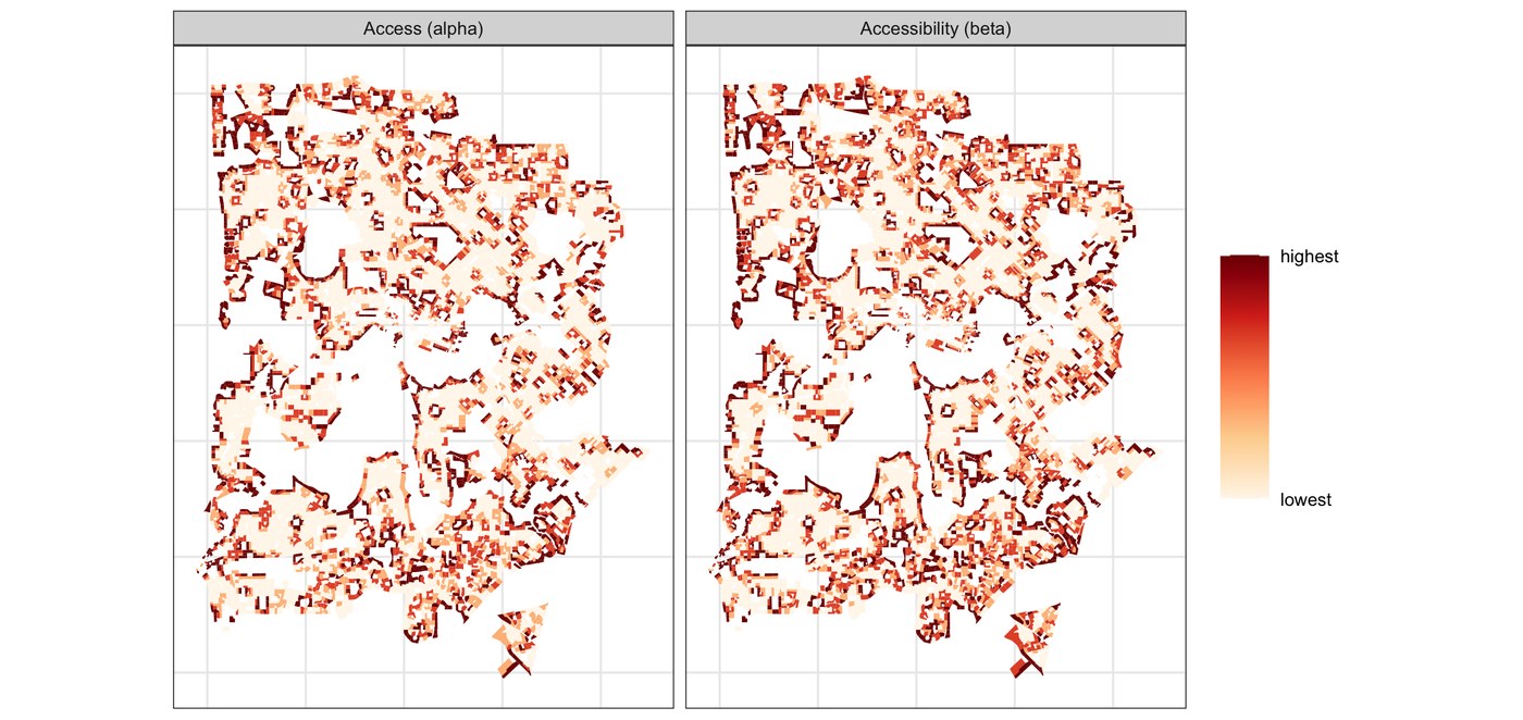
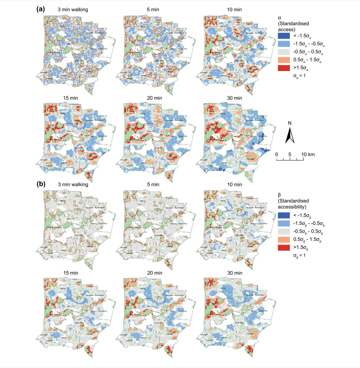
The published findings are recovered — checked
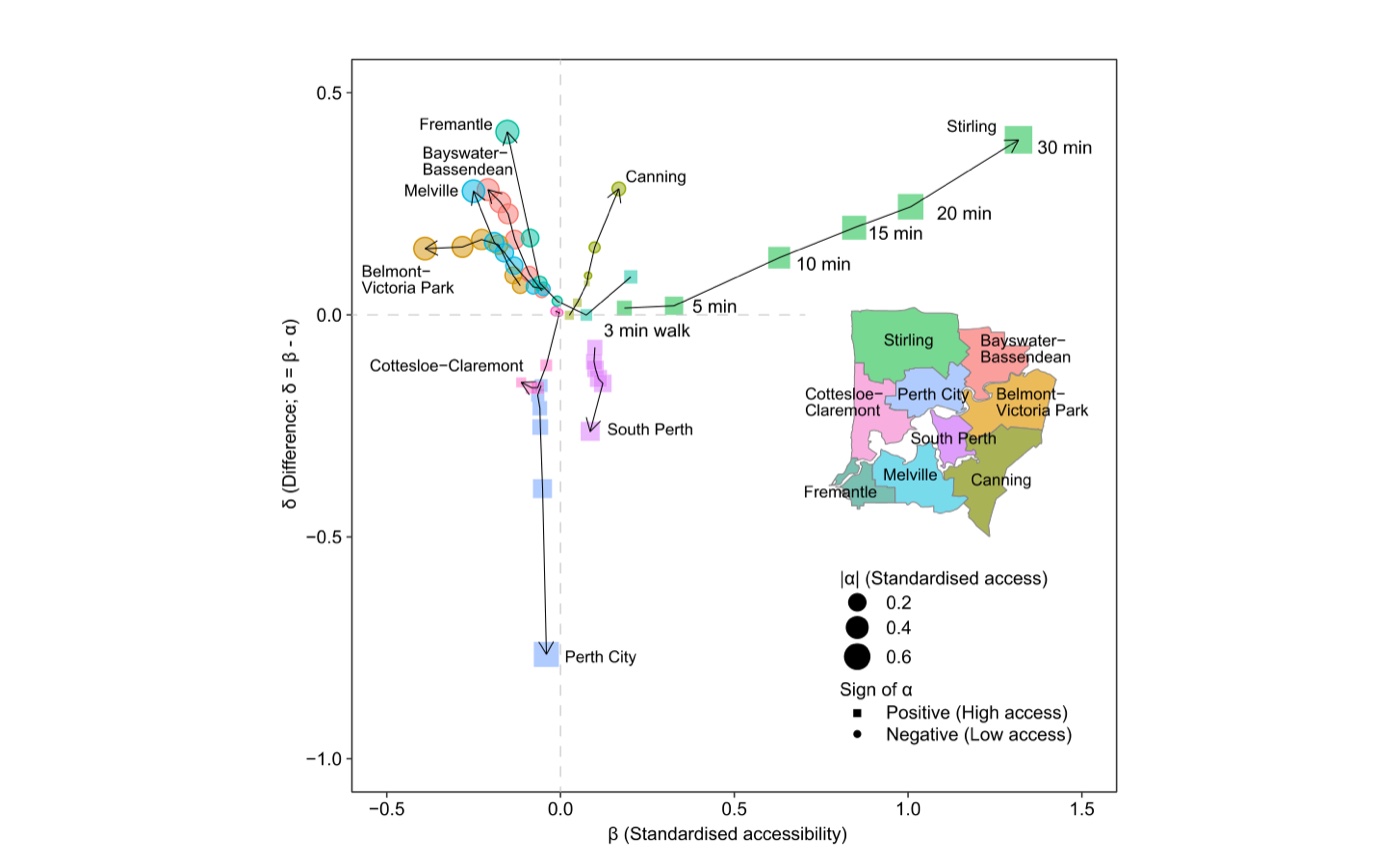
The regional pattern falls out of the analysis rather than being asserted. At a 30-minute walk the demo puts Perth City lowest at δ = −0.765 and Fremantle highest at +0.412 — the two extremes of the paper's Fig. 5, at the values its axis shows (reproduced in §1.1).
The measurement of α and β is demonstrated, not reproduced — stated plainly
Step 2 recomputes both measures from the block geometry. Against the published columns, access correlates at r = 0.61 and accessibility at r = −0.08. The reason is §2.4: the published β is built on road-network distances, and the demonstration uses straight lines. The demonstration is faithful to the practical tutorial — it reproduces that document's printed median of 0.0105 — but it is not the paper's β, and nothing downstream uses it.
== test-01  The published analysis table ================================
   8259 residential blocks, as published                      pass
   nine SA3 regions                                           pass
   six walking times are present                              pass
   delta = accessibility - access at every scale (max dev 1.0e-06) pass
   access at  3 min is standardised (mean -0.00, sd 1.00)     pass
   access at 30 min is standardised (mean -0.00, sd 1.00)     pass
   six raw explanatory variables are present                  pass
   six contextualised variables are present                   pass
   every analysis row matches a residential block (8259 of 8259) pass
   providers are present in the geometry                      pass
   10 passed, 0 failed
   PASS - the published analysis table is intact

== test-02  Model properties ============================================
   delta is positive exactly when accessibility exceeds access pass
   adding a constant to both leaves delta unchanged           pass
   delta changes sign when the two measures are swapped       pass
   perfectly separated strata give PD near 1 (1.000)          pass
   meaningless strata give PD near 0 (0.004)                  pass
   no terminal node is smaller than minbucket (smallest 45)   pass
   distances follow 5 km/h to within 5 m                      pass
   ...
   11 passed, 0 failed
3.3 Core Analytical Steps
Five stages: purpose → code → output → result → how to read it.
Prepare data — and check the identity the model rests on
What this step does
Reads the analysis table and the block geometry, records what each column is, and confirms that δ really is β − α at every walking time. That check is cheap and it is the one thing that must be true for anything downstream to mean what it says.
Code
d <- read_analysis()

# The identity the whole model rests on: delta must be beta - alpha
# at every walking time, or nothing downstream means what it says.
worst <- 0
for (t in WALK_TIMES) {
  dev   <- max(abs(d[[col_delta(t)]] -
                   (d[[col_accessibility(t)]] - d[[col_access(t)]])))
  worst <- max(worst, dev)
}
if (worst > 1e-4) log_warn("delta does not match beta - alpha; check the input table")
Example output
== Step 1/5  Prepare data ======================================
   analysis table: 8259 residential blocks, 47 columns
   regions: 9 (Bayswater-Bassendean, Belmont-Victoria Park, Canning ...)
   scales: 3/5/10/15/20/30 minutes (250/417/833/1250/1667/2500 m) at 5 km/h
   delta = accessibility - access holds to 1.0e-06 across all scales
   geometry: 9449 blocks (8276 Residential, 1173 Parkland)
joined 8259 of 8259 analysis rows to geometry- 8,276 consumers and 1,173 providers. Residential blocks demand greenspace; parkland blocks supply it. Every accessibility model needs that split stated explicitly, because it decides what the model can see.
- The identity is checked, not assumed. If δ and β − α ever drift apart, some column has been transformed or misaligned, and every later number is quietly wrong.
Where access and accessibility come from
What this step does
Recomputes both measures from the geometry, so the two definitions are concrete rather than assumed. Access is a sum of supply within reach; accessibility is a floating catchment ratio that discounts supply by distance and divides it by the population competing for it.
Code
# access: the greenspace area within the walking distance
D <- sf::st_distance(consumer_centroids, provider_centroids)
alpha <- as.numeric((D <= d0) %*% providers$AREASQKM21)

# accessibility: MG2SFCA — supply discounted by distance, shared among demand
beta <- catchment::catchment_ratio(
  consumers = consumer_centroids, providers = provider_centroids,
  weight = "gaussian", consumers_value = "Person",
  providers_value = "AREASQKM21", max_cost = d0, return_type = "region")
Example output
== Step 2/5  How access and accessibility are computed =========
   demonstrating at 3 minutes = 250 m (5 km/h)
   consumers: 8276 Residential blocks | providers: 1173 Parkland blocks
   access: greenspace area within 250 m; 34.6% of blocks reach any greenspace
   at this distance most blocks reach none, so access is zero for them —
   a short walking time makes access a coarse, mostly-empty measure
   access among blocks that reach some: median 0.0207 km2
   accessibility: MG2SFCA with a Gaussian decay, median 0.010483
against the published columns: access r = 0.606, accessibility r = -0.076- Access is coarse at short distances, and that is the point. Within 250 m only 35% of blocks reach any greenspace at all; for the rest access is simply zero. A measure that is zero for two thirds of a city cannot distinguish between them — which is the gap accessibility is designed to fill.
- Accessibility is never zero in the same way. The floating catchment discounts distant supply rather than discarding it, so it grades where access only counts.
- The correlation against the published β is −0.08, and that number is the lesson. Swapping network distances for straight lines does not perturb the measure slightly; it produces a different measure. If you cannot build the network, say so in the methods — do not present Euclidean accessibility as though it were the same quantity.
The delta, and the green-city classification
What this step does
Differences the two standardised measures at each walking time, classifies every block by the sign of the result, and summarises by region. The near-zero class needs a band rather than an exact value, since δ is continuous: one tenth of a standard deviation, which keeps the classification comparable across scales.
Code
a <- d[[col_access(t)]]; b <- d[[col_accessibility(t)]]; dl <- d[[col_delta(t)]]

# Summarise the difference at each walking time
data.frame(walk_minutes = t,
           mean_delta     = mean(dl),
           share_positive = mean(dl > 0),
           share_negative = mean(dl < 0),
           cor_access_accessibility = stats::cor(a, b))

# The green-city classification: a band of width sd/10 around zero is "zero"
eps <- stats::sd(dl) / 10
k   <- ifelse(dl > eps, "positive", ifelse(dl < -eps, "negative", "zero"))
Example output
| Walk | Distance | δ > 0 | δ ≈ 0 | δ < 0 | cor(α, β) |
|---|---|---|---|---|---|
| 3 min | 250 m | 55.7% | 8.3% | 36.0% | +0.749 |
| 5 min | 417 m | 52.1% | 10.9% | 37.0% | +0.716 |
| 10 min | 833 m | 51.1% | 10.6% | 38.3% | +0.745 |
| 15 min | 1250 m | 49.1% | 11.9% | 39.0% | +0.709 |
| 20 min | 1667 m | 47.2% | 10.4% | 42.4% | +0.711 |
| 30 min | 2500 m | 43.2% | 9.6% | 47.2% | +0.680 |
results/green-city-classification.csv and
delta-summary.csv. The majority flips: at a three-minute walk most blocks have
accessibility ahead of access; at thirty minutes most have fallen behind.
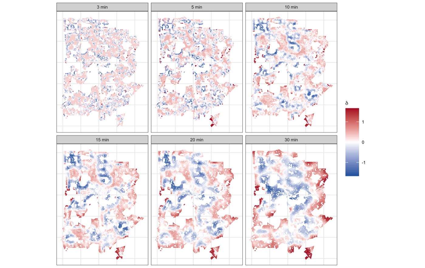
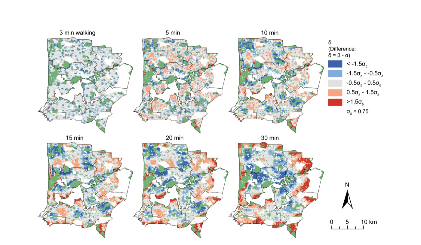
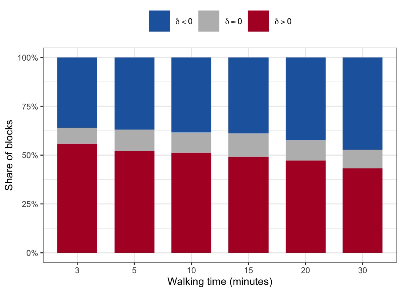
- The crossover is the headline. Positive blocks fall from 55.7% to 43.2% as the walk lengthens, and negative ones rise past them. Close to home, Perth's greenspace is easier to use than its bare quantity suggests; over a half-hour walk the opposite holds. A single-distance study would have found one of these and missed that it reverses.
- α and β correlate at about +0.7, not +1. They are measuring related things — which is why differencing them is meaningful rather than trivial — but roughly half the variance is not shared, and that half is what δ isolates.
- Perth City is the clearest case. Lowest δ at every scale, reaching −0.765 at thirty minutes: the city centre has greenspace, but it is distant, contested and hard to reach relative to how much is nominally there.
- The near-zero band is a choice, so it is stated. One tenth of a standard deviation; about a tenth of blocks land in it. Widen it and the story becomes "mostly neutral", narrow it and the neutral class vanishes — report whichever you use.
What explains the difference
What this step does
Each variable is cut into spatial strata by a regression tree, and the geographical detector scores how much of δ those strata explain. Every variable is tested twice: as its own value, and in a contextualised form carrying its local spatial pattern.
Code
# the variable is continuous, so a tree turns it into spatial strata
tr <- rpart::rpart(df ~ v, data = dd, minbucket = TREE_MINBUCKET)
dd$strata <- as.character(as.numeric(tr$where))

# then the detector scores how much of delta those strata account for
g <- GD::gd(df ~ strata, dd)      # g$Factor$qv is the Power of Determinant
Example output
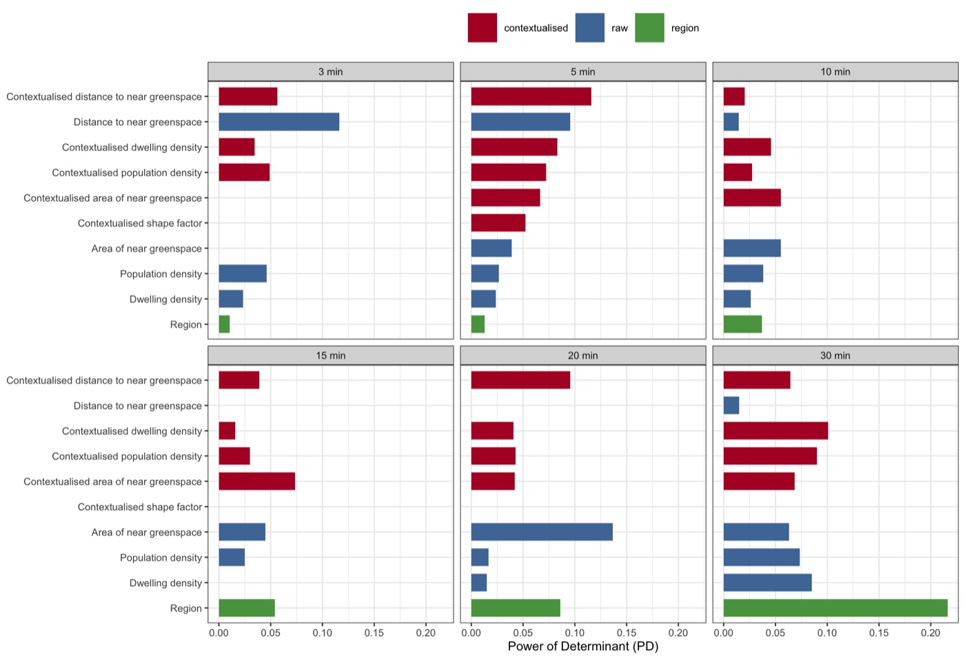
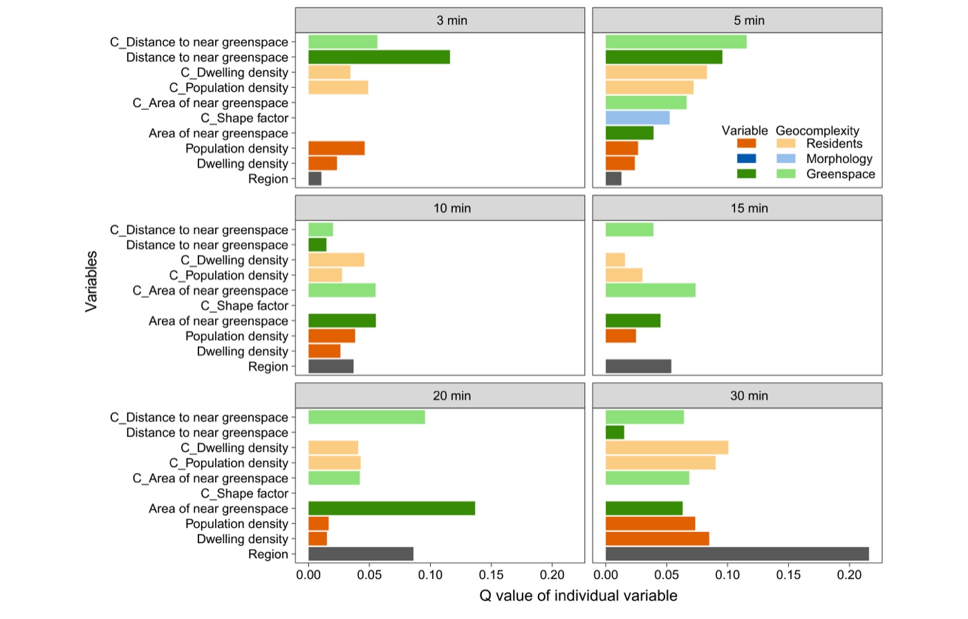
| Walk | Strongest single variable | PD | All variables jointly |
|---|---|---|---|
| 3 min | Distance to near greenspace (raw) | 0.116 | 0.262 |
| 5 min | Distance to near greenspace (contextualised) | 0.116 | 0.235 |
| 10 min | Area of near greenspace (raw) | 0.055 | 0.197 |
| 15 min | Area of near greenspace (contextualised) | 0.074 | 0.272 |
| 20 min | Area of near greenspace (raw) | 0.137 | 0.250 |
| 30 min | Region | 0.216 | 0.426 |
results/drivers-pd.csv and drivers-total-pd.csv.
- What drives the gap changes with the distance considered. At a three-minute walk it is how far the nearest park is. By thirty minutes the strongest single predictor is simply which region you are in (PD 0.216) — at that range the difference is a property of urban structure at the district scale, not of the individual block.
- Arrangement often beats quantity. The contextualised forms outscore their raw counterparts at four of the six scales. How greenspace and population are patterned around a block explains the access–accessibility gap better than how much of each there is — which is what the difference was built to capture.
- Together they explain a fifth to two fifths. Jointly, PD runs 0.197 to 0.426, highest at thirty minutes. Most of δ remains unexplained by these twelve variables, and reporting that honestly is better than implying the gap is solved.
- Region is weak at short range and dominant at long. PD 0.013 at five minutes against 0.216 at thirty: administrative geography says almost nothing about your walk to the nearest park, and a great deal about your access to the city's greenspace as a whole.
Interactions — pairs that explain more together
What this step does
Overlays each pair of stratifications and scores the combined zones, classifying the pair into the five standard interaction types.
Code
# Each variable becomes spatial strata through a tree fitted against delta
strata_of <- function(x) {
  if (is.character(x) || is.factor(x)) return(as.character(x))
  tr <- rpart::rpart(df ~ v, data = data.frame(df = y, v = x),
                     minbucket = TREE_MINBUCKET)
  as.character(as.numeric(tr$where))
}

# Power of Determinant of one stratification, and of a pair combined
pd_strata <- function(s)
  as.numeric(GD::gd(df ~ strata, data.frame(df = y, strata = s))$Factor$qv)

single <- vapply(lapply(vars, strata_of), pd_strata, numeric(1))
Example output
| Variable 1 | Variable 2 | PD₁ | PD₂ | PID | Type |
|---|---|---|---|---|---|
| Area of near greenspace | Contextualised population density | 0.039 | 0.072 | 0.282 | Enhance, nonlinear |
| Region | Contextualised distance to near greenspace | 0.013 | 0.116 | 0.248 | Enhance, nonlinear |
| Contextualised dwelling density | Contextualised distance to near greenspace | 0.083 | 0.116 | 0.208 | Enhance, nonlinear |
results/interaction-pid.csv at a 5-minute walk, strongest three of
45 pairs. Of the 45, 28 are nonlinear-enhance, 13 bi-enhance and 4 uni-weaken.
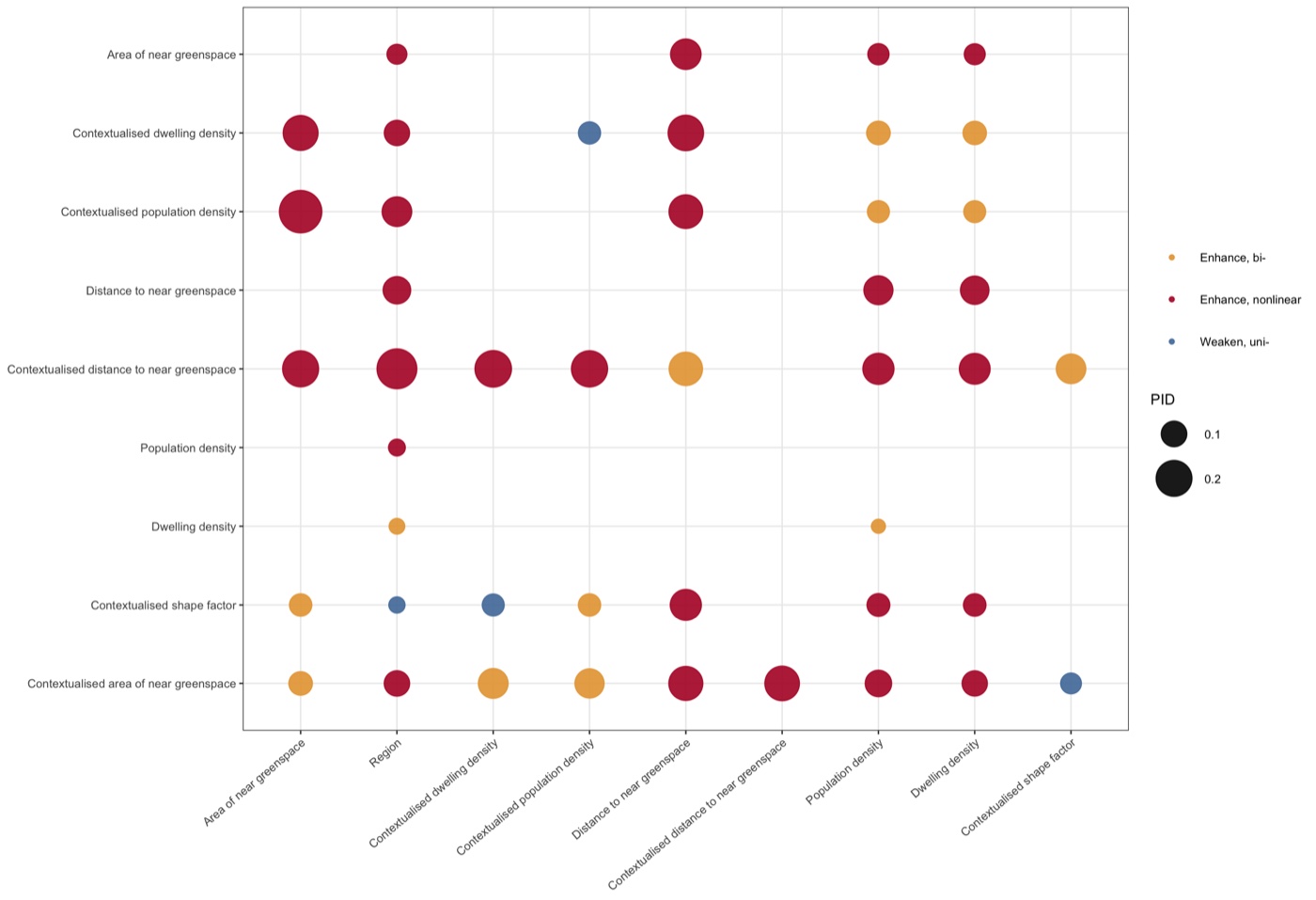
- The best pair more than doubles the best single. PID 0.282 against a strongest single PD of 0.116 — a gain of 144%. Greenspace area and population pattern say far more about the gap jointly than either says alone, which is exactly what you would expect of a measure built from supply and competition.
- Nonlinear-enhance dominates: 28 of 45 pairs. The joint effect exceeds the sum of the parts. These variables are not independent contributions to be added up; they condition each other.
- Region is weak alone but strong in company. PD 0.013 by itself, PID 0.248 paired with contextualised distance — the district matters, but only once you know the local greenspace geography within it.
3.4 Reading the Results Together
| The gap is real | α and β correlate at only ~0.7, and 37–47% of blocks have accessibility falling short of access. |
|---|---|
| It reverses with distance | 55.7% of blocks are positive at a 3-minute walk, 43.2% at 30 — the majority flips. |
| And it is explainable | Jointly PD 0.20–0.43; nearest-greenspace geometry rules the short walk, region the long one. |
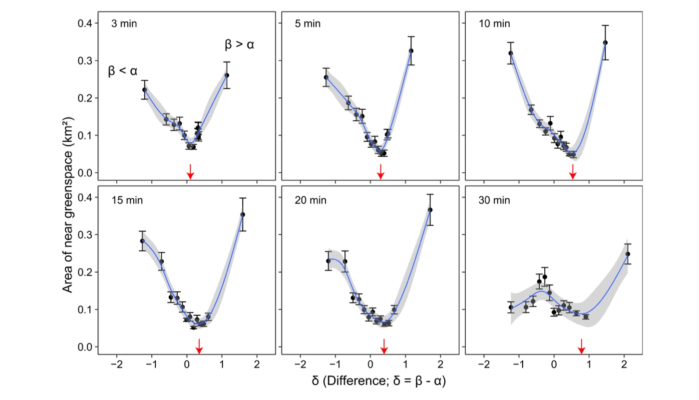
- Mechanism. Access counts supply; accessibility divides discounted supply by the demand competing for it. So δ is negative wherever greenspace is distant, obstructed or crowded relative to its quantity, and positive where a modest amount of parkland is close, unobstructed and lightly shared. The gap is a statement about urban form, not about hectares.
- Why the reversal matters for policy. Near home, Perth's greenspace works better than its quantity implies; at half an hour it works worse. A programme judged at one distance can look like a success or a failure depending on a choice nobody examined — so report the whole curve, as the model does.
- Decision angle. Negative δ and low α call for new greenspace. Negative δ with high α calls for something else entirely — crossings, paths, entrances, maintenance — because the hectares are already there. Distinguishing those two cases is the practical payoff, and neither α nor β alone can do it.
- What SDM is not. It is not a measure of greenspace quality, and δ near zero is not a clean bill of health: it means the two measures agree, which can happen in a place with plenty of easily-reached parkland or with almost none. Read δ next to α, as the paper's Fig. 5 does, not on its own.
- Honest limits. The published β needs road-network distances that are built by hand (§2.4); the demonstration here uses straight lines and correlates at −0.08 with the published values, which is the size of the error that shortcut introduces. Twelve variables explain at most 43% of δ. And the classification's neutral band is a convention, not a finding.
1) Step 1's identity check — δ must equal β − α, or nothing else counts.
2) results/delta-summary.csv — how far α and β actually diverge, and whether the
balance shifts with distance. 3) results/delta-by-region.csv — which places sit
at the extremes, and whether that is plausible on the ground.
4) results/drivers-pd.csv — what explains the gap, and whether arrangement beats
quantity. 5) results/interaction-pid.csv — which pairs act together.
4 Adaptation, Writing & Reproducibility
4.1 Port to Your Domain
Nothing in the model is specific to greenspace. It needs a service that people travel to, a population that travels to it, and a way of measuring the journey. Swap those three and the method is unchanged:
| Domain | Consumers | Providers | What δ would mean |
|---|---|---|---|
| Urban greenspace (this demo) | residential blocks, by population | parkland, by area | parks that exist but cannot be used |
| Primary healthcare | population by age band | clinics, by capacity | coverage on paper versus in practice |
| Schools | school-age children | schools, by places | catchments that look adequate but are not |
| Food retail | households | supermarkets, by floorspace | food deserts hidden by nominal proximity |
Any supply–demand pair with a travel cost between them fits the contract of §2.3.
What to edit
config/project-config.R— the three data paths,ID_COLandREGION_COL, and the consumer and provider categories with their demand and supply fields.WALK_TIMESandWALK_DISTANCES— the scales that matter for your service. A clinic is not a park: the relevant range may be a drive rather than a walk, in which case set the distances from the appropriate speed and say so.VARS_RAWandVARS_CTX— the candidate explanations, in both plain and contextualised form if you have them.- Compute α and β for your own case (Step 2 shows the shape of it; §2.4 covers the network distances), write them into the analysis table under the configured prefixes, and the rest of the pipeline runs unchanged.
Standardise α and β before differencing — they are an area and a ratio, and subtracting them raw is meaningless. Keep identifier columns as text, or long numeric codes will silently fail to join. Do not read δ without α beside it: zero means "the two agree", which is a very different situation in a park-rich suburb than in a park-poor one. Report the walking-time curve rather than one distance, because the balance genuinely reverses. And if you use straight-line distances, state it — §3.2 shows what that costs.
4.2 Write the Paper
| Manuscript section | Template output | Writing job |
|---|---|---|
| Methods | config/project-config.R, results/walking-scales.csv | define access and accessibility with their formulas, state the walking times and the speed behind them, the distance basis (network or straight-line), and the standardisation before differencing |
| Results | figs/fig01–fig06, tables/table-delta-summary.tex, table-drivers-pd.tex | map α and β, then δ; report the classification across scales including the crossover; then the drivers and their interactions; every finding sentence carries a number |
| Discussion | results/delta-by-region.csv, drivers-total-pd.csv | argue what a negative δ implies for policy where α is high versus low, and how much of the gap remains unexplained |
Where each manuscript section draws its material from.
Manuscript skeleton
1  Introduction        — access is not accessibility; why the gap matters;
                          the contribution (3 aims)
2  Spatial Delta Model — 2.1 Access (alpha): supply within reach
                          2.2 Accessibility (beta): MG2SFCA, all formulas here
                          2.3 The difference (delta) and its interpretation
                          2.4 Spatial scales, and the distance basis
3  Case & data         — study area, consumers, providers, explanatory variables
4  Results             — 4.1 access and accessibility mapped
                          4.2 the difference, and how it changes with distance
                          4.3 the green-city classification by region
                          4.4 what explains the difference (PD by scale)
                          4.5 interactions between explanations
5  Discussion          — high-alpha vs low-alpha negatives; the scale reversal;
                          what remains unexplained; distance-basis limitations
6  Conclusions         — 6-8 sentences answering the aims
Results-to-manuscript map
| Manuscript element | Source file | Shown in |
|---|---|---|
| Access and accessibility maps | figs/fig01 | §4.1 |
| Main figure (δ across scales) | figs/fig02 | §4.2 |
| The α–β plane | figs/fig03 | §4.2 |
| Classification shares | figs/fig04, tables/table-classification.tex | §4.3 |
| Drivers by scale | figs/fig05, tables/table-drivers-pd.tex | §4.4 |
| Interactions | figs/fig06, tables/table-interactions.tex | §4.5 |
Every manuscript element traces to one regenerable file.
4.3 Final Reproducibility Package
| Code | numbered scripts in R/ + run-all.R + config/project-config.R + tests/ |
|---|---|
| Data | data/mbvars.csv, blocks.gpkg, regions.gpkg, with provenance.md |
| Results | figs/fig01–fig06 + tables/*.tex + env/session-info.txt |
Rscript run-all.R testpasses — 21 checks, including the model identity at every scale and the full 8,259-row join.- Delete
results/,tables/,figs/anddata/derived/, re-runRscript run-all.R— every number and figure on this page regenerates (~15 s). - The walking times, the speed behind the distances, the distance basis
(network or straight-line) and the tree's minimum node size are stated in the
manuscript and match
config/project-config.R. - α and β are reported as standardised, and the classification's neutral band is defined.
env/session-info.txtis included in the deposit.
Isn't δ just noise from two noisy measures? → no: α and β correlate at ~0.7, δ is
spatially organised (figs/fig02), and a fifth to two fifths of it is explained
by measurable urban form. Why that walking time? → all six are reported, and the
balance reverses between them. Euclidean or network distance? → §2.4, and §3.2 shows
the −0.08 correlation that shortcut produces. Is the neutral class arbitrary? → yes,
it is a convention; it is defined and its width stated. Does region just proxy for
everything? → no: PD 0.013 at five minutes, 0.216 at thirty.
References & credits
Demo outputs were generated by the scripts in this folder from the authors' own analysis table. Reference figures are reproduced from the article, which is open access under CC BY, and from the accompanying practical tutorial.
- Lin G, Song Y, Xu D, Swapan MSH, Wu P, Hou W, Xiao Z (2024). Interpreting differences in access and accessibility to urban greenspace through geospatial analysis. International Journal of Applied Earth Observation and Geoinformation 129:103823. doi:10.1016/j.jag.2024.103823 · PDF (source of the method, the case data, and the Fig. 1, 3, 4, 5, 6 and 7 reference images)
- Delamater PL (2013). Spatial accessibility in suboptimally configured healthcare systems: a modified two-step floating catchment area (M2SFCA) metric. Health & Place 24:30–43. doi:10.1016/j.healthplace.2013.07.012 (the accessibility model behind β)
- Song Y, Wang J, Ge Y, Xu C (2020). An optimal parameters-based geographical detector model. GIScience & Remote Sensing 57(5):593–610. doi:10.1080/15481603.2020.1760434 · OPGD tutorial (the detector used in Steps 4 and 5)
- The
catchmentR package (Social and Decision Analytics Division, University of Virginia) — used for the MG2SFCA demonstration in Step 2.