Reproducible models · Tutorial 11 of 13
Reproducing the Singularity Regression Kriging (SRK) Model
A complete walkthrough of the SRK model — which measures how a covariate's local intensity scales with neighbourhood size, feeds that singularity index to a random forest as an extra predictor, and kriges what the forest leaves behind — from raw geochemical samples to manuscript. The method is implemented here in a single self-contained R file, reproduced on the paper's own simulation and on its 998 cobalt samples from Western Australia, and stress-tested with an error bar the published comparison does not carry.
To cite the SRK model in publications, please use:
Ren K, Song Y*, Chen M, Yu Q (2026). A singularity regression kriging for spatial prediction. GIScience & Remote Sensing 63(1):2690341. doi · PDFCC BY · authors' code
R/ pipeline scripts including the complete method in R/02-srk-core.R · config/project-config.R · results/ and tables/ (every number quoted on this page) · tests/ · run-all.R — unzip and run Rscript run-all.R from the SRK/ folder root. The case-study sample table is downloaded by the pipeline, not bundled; see §2.4.
1 Method Overview & Reproduction Scope
1.1 Core Idea
Regression kriging splits a spatial variable into a deterministic trend and a spatially correlated residual, predicts the trend from covariates, and kriges the rest. The weak link is the trend model. Ordinary kriging (OK) assumes there is no trend at all — a constant mean — and regression kriging usually assumes a linear one. Both leave nonlinear, multiscale structure sitting in the residual, where a variogram fitted under an assumption of stationarity cannot represent it.
Ren et al. (2026) change exactly one thing: what the trend model is allowed to see. Alongside each environmental covariate Xk they compute its singularity index αk(s) — the exponent describing how the local intensity of that covariate scales as the measuring window grows. A value of 2 means the field is locally uniform; below 2 means local enrichment; above 2 means depletion. The random forest is then trained on the covariates and their singularity indices, and ordinary kriging is applied to what the forest still cannot explain.
- Research problem: in heterogeneous terrain the response is nonlinear, multiscale and non-Gaussian, so a kriging model with a simple trend degrades exactly where the interesting anomalies are.
- One-line contribution: SRK builds anomaly descriptors from the covariates at a ladder of spatial scales, hands them to the trend model, and leaves the residual closer to stationary — which is what the kriging step assumes in the first place.
- Why the covariate, not the response, matters: a singularity index built from the response could only be evaluated where the response is known — that is, never at a prediction location, and never inside a held-out block. Building it from covariates is what lets the feature survive spatial block cross-validation instead of leaking through it.
- What it buys: on the paper's simulation, reproduced below, SRK lifts R2 from 0.876 to 0.972 on a near-normal field, and from 0.736 to 0.940 on a long-tailed one — the margin widens as the distribution departs from Gaussian. On the real cobalt data it lifts R2 from 0.15 (ordinary kriging) to 0.36 under spatial blocking, and stays ahead of the strongest machine-learning benchmark on every one of 20 random-forest seeds (§3.2 Step 5).
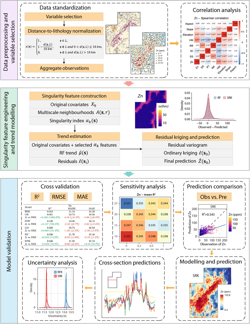
One covariate, measured in windows of growing size, gives one number per location: the slope of log intensity against log scale, plus two. That number is a new column. The forest gets it, the residual gets smaller, the kriging step gets an easier job. Everything on this page serves that line.
R 4.1+ and the folder from the download button. The method itself is
R/02-srk-core.R, about 250 lines that depend on four packages:
ranger for the forest, automap and gstat for
the variogram and kriging, sp for coordinate handling. The singularity
indices, the variance filter, the spatial block folds and the accuracy metrics are
base R. The full pipeline runs in about two and a half minutes, most of it in the
two robustness steps.
1.2 Method Logic (Eq. 1–13)
SRK chains three standard tools in a specific order. Each link is simple; the model is what the middle one is given to work with.
Key concepts and equations
- Local covariate intensity (Eq. 2). At location s and scale
r, take the mean absolute covariate value over every reference point inside
the square window A(s, r):
Ĉk(A(s, r)) = (1 / |A(s, r)|) Σs′ ∈ A(s,r) |Xk(s′)|(2)A scale carrying fewer than three reference points is discarded, not guessed at.
- The scaling law and the index (Eq. 1, 3–4). Across scales
r1 < … < rJ the
theoretical relation C ∝ rα−2
becomes a straight line in logarithms, and α is its slope plus two:
log Ĉk(A(s,r)) = (αk(s) − 2) log r + ck(s) + ek,r αk(s) = β̂1,k(s) + 2(3–4)α = 2 is a spatially uniform field, α < 2 is local enrichment, α > 2 is local depletion. Locations with fewer than two usable scales are set to the neutral 2.
- The augmented feature set (Eq. 5). The q singularity columns
that survive the SD filter join the p original covariates:
F(si) = { X1(si), …, Xp(si), αk1(si), …, αkq(si) }(5)
- Trend and residual (Eq. 6–7). A 500-tree random forest
g(·) fits the trend, and the residual is what it misses:
µ̂(si) = g(F(si)) ε(si) = Z(si) − µ̂(si)(6–7)
- Residual kriging and the final prediction (Eq. 8–10). Ordinary
kriging interpolates ε under the unbiasedness constraint, and the two parts
are added:
Ẑ(s0) = µ̂(s0) + Σi λi ε(si), Σi λi = 1 δ(s0) = √σK2(s0)(8–10)The kriging standard error δ is the model's uncertainty measure.
- Accuracy (Eq. 11–13). R2, RMSE and MAE on the held-out validation data, never on the training fit.
The window is a square of half-width r — the Chebyshev ball, not a disc — and the reference points inside it are the sample locations, not a raster. So C(A(s, r)) is a mean over however many observations of the covariate happen to fall within r in both easting and northing. That is why the sampling design shows through in the index, and why a minimum count per scale is part of the definition rather than an implementation detail.
1.3 Reproduction Scope
This pipeline reproduces the paper's simulation experiment and its
case study up to spatial block cross-validation. The article maps two trace
elements; this tutorial follows cobalt end to end, because every step is written
as a loop over the ELEMENTS list and one element is enough to show each
step working — putting zinc back is a single config entry
(§2.3). Everything tagged Demo run regenerates
from the folder behind the download button; everything tagged Published reference
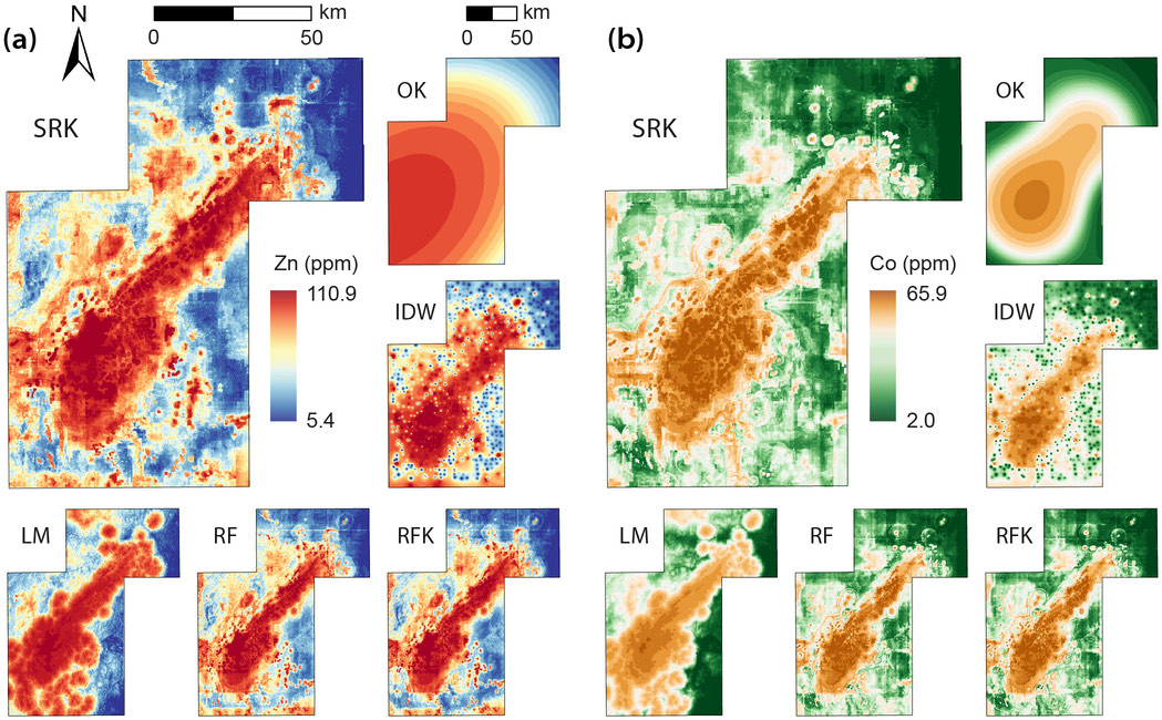
is a static image from the article. The published prediction maps, cross-sections and
uncertainty maps need the 97,234-cell 500 m prediction grid, which is out of scope
here; §3.3 shows those figures from the article and says what
it would take to regenerate them.
| Item | This pipeline | Published article |
|---|---|---|
| Simulation | Same 20 × 20 grid, same spherical fields, same seed 42, same 70/30 split — Table 1 reproduced to three decimals | Sec. 2.3, Table 1, Figs. 1–2 |
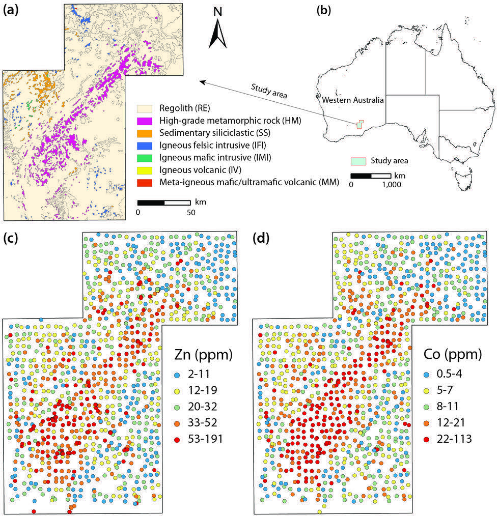
| Case-study samples | The authors' released table: 998 Co samples with four lithology proximity
variables and three terrain variables, downloaded by
R/20-case-data.R |
Zn (n = 1,105) and Co (n = 998) from GSWA geochemistry (DMIRS-047) with Geoscience Australia lithology and DEM, Sec. 3.1 |
| Covariate screening | Spearman screen re-run from the data; it returns the published covariate set | Sec. 4.2, Fig. 5 |
| Singularity features | 2–20 km at 2 km steps, ≥ 3 neighbours per scale, ≥ 2 valid scales, SD > 0.5 filter | Sec. 3.2.2, Sec. 4.3, Fig. 6 |
| Validation | 5-fold spatial block CV, 15 km blocks, six models — the Co half of Table 2 reproduced, with the deterministic rows exact | Sec. 3.2.3, Table 2, Fig. 8 |
| Sensitivity | Maximum scale × SD threshold grid, 30 cells | Sec. 4.4, Fig. 7 |
| Seed stability | Added here. The same cross-validation repeated over 20 random forest seeds, because the released scripts fix none | not in the article |
| Full-grid prediction | out of scope — needs the 8.1 MB, 97,234-cell grid | Figs. 9–11 |
1.4 Which Implementation This Page Follows
Two bodies of R code carry the SRK name, and they are not the same thing.
| The authors' scripts | CRAN SingRegKrig 0.1.0 | |
|---|---|---|
| Written by | Ren, Song, Chen and Yu — the paper's authors (GitHub, Figshare) | Tyagi, Pandey, Singh and Tripathi — an independent third-party implementation that cites the paper; none of the paper's authors is an author of the package |
| Engine | ranger + automap::autoKrige, with a hand-written
singularity.R |
randomForest + gstat, with its own
compute_singularity() |
| Reproduces the article's numbers | Yes — this page does it below | No. Its bundled sim_srk_data() is a different generator, and
on it SRK does not reach the article's Table 1 |
sd_threshold firstsrk() defaults to sd_threshold = 0.5, the value the
article uses for lithology proximity variables whose singularity indices have
SD of 6 or more. On the package's own simulated data the single singularity feature
has SD = 0.29, so the default discards it: retained_features
comes back as character(0) and the fitted model is random-forest
kriging with no singularity term at all. The filter is doing what it was designed to
do; the default is simply calibrated to a different kind of covariate. Inspect
fit$retained_features before reporting anything as an SRK result.
This page follows the authors' scripts. R/02-srk-core.R is a port of
them into the step-numbered layout the rest of this tutorial series uses, and every
place it departs from them is marked DEPARTURE in the source and listed in
§2.2.
2 Setup, Code & Data
2.1 Environment & Dependencies
Four packages, all on CRAN. Nothing else is needed: the singularity indices, the variance filter, the spatial block folds, the accuracy metrics and every figure are base R.
install.packages(c("sp", "gstat", "automap", "ranger"))| Package | Used for | Where |
|---|---|---|
ranger | the 500-tree random forest trend model | srk_trend() |
automap | autoKrige — automatic variogram family choice and ordinary kriging, exactly as the paper specifies | srk_krige_residuals(), bench_ok() |
gstat | unconditional Gaussian simulation of the two base fields; the IDW benchmark | R/10-simulate.R, bench_idw() |
sp | coordinate promotion for the two above | throughout |
Verified on R 4.6.0. Runtimes and the one known version sensitivity
are in env/requirements.md.
2.2 The Method in One File
R/02-srk-core.R holds the whole model. Three functions carry
Eq. 1–10; everything else in the file is the five benchmarks, the metrics and the
block folds, which exist so the cross-validation loop can treat all six models
identically.
Eq. 2 — local intensity at every scale, in one pass
The authors' singularity_safe() loops over evaluation points and scales.
The port keeps the definition and vectorises the search: one Chebyshev distance matrix
per chunk of evaluation points, then one logical mask per scale. That is what makes the
sensitivity analysis in step 6 affordable — the intensity matrix is computed once
and re-cut for every shorter scale ladder.
srk_intensity <- function(x_ref, y_ref, z_ref, x_eval, y_eval, scales,
                          min_pts_per_scale = 3L, use_abs = TRUE,
                          chunk = 2000L) {
  if (use_abs) z_ref <- abs(z_ref)
  n_eval <- length(x_eval)
  J      <- length(scales)
  C      <- matrix(NA_real_, n_eval, J)
  # Chunked so a large evaluation set never allocates one huge distance matrix.
  for (ii in split(seq_len(n_eval), ceiling(seq_len(n_eval) / chunk))) {
    d <- pmax(abs(outer(x_eval[ii], x_ref, "-")),
              abs(outer(y_eval[ii], y_ref, "-")))    # square window = Chebyshev ball
    for (j in seq_len(J)) {
      inw <- d <= scales[j]
      cnt <- rowSums(inw)
      val <- as.numeric(inw %*% z_ref) / cnt
      val[cnt < min_pts_per_scale] <- NA_real_       # too few neighbours: no estimate
      C[ii, j] <- val
    }
  }
  C
}
Eq. 3–4 — the index is a slope plus two
srk_alpha <- function(C, scales, min_valid_scales = 2L, eps = 1e-9) {
  logr <- log(scales)
  vapply(seq_len(nrow(C)), function(i) {
    cr <- C[i, ]
    ok <- is.finite(cr)
    if (sum(ok) < min_valid_scales) return(NA_real_)   # caller substitutes 2
    yv <- log(ifelse(cr[ok] > 0, cr[ok], eps))         # a window of zeros is possible
    xv <- logr[ok]
    xd <- xv - mean(xv)
    sum(xd * (yv - mean(yv))) / sum(xd * xd) + 2
  }, numeric(1))
}
tests/test-01 transcribes the authors' loop verbatim and checks that
these two functions return the same numbers to 1e−10, including which locations
come back as NA.
Eq. 5–9 — the model
srk_run() is the whole method: build or look up the singularity columns,
drop the flat ones, fit the forest, krige what is left, add the two together. It shares
its argument list with the five benchmarks, so SRK_MODELS can be iterated
over.
srk_run <- function(train, test, yvar, xvars, sv = NULL, ...) {

  ## Step 1 — one singularity column per covariate (Eq. 1-4).
  ##   Covariates are observable at prediction locations, so the union of train
  ##   and test may supply the reference values without leaking the response.
  ...
  for (cc in sv_cols) {
    tr[[cc]][!is.finite(tr[[cc]])] <- neutral          # 2 = uniform field
    te[[cc]][!is.finite(te[[cc]])] <- neutral
  }

  ## Step 2 — variance filter, then the forest (Eq. 5-7).
  sv_keep <- srk_select_features(tr, sv_cols, sd_threshold)
  tri     <- srk_trend(tr, te, yvar, c(xvars, sv_keep), ntree = ntree,
                       seed = seed, use_coords = use_coords)
  tr$resid <- tr[[yvar]] - tri$trend_tr

  ## Step 3 — ordinary kriging of the residual, added back (Eq. 8-9).
  kr <- srk_krige_residuals(tr, te, "resid", fitter = fitter)

  list(model = "SRK", pred = tri$trend_te + kr$pred, trend = tri$trend_te,
       kriged = kr$pred, se = kr$se, sv_kept = sv_keep, ...)
}

SRK_MODELS <- list(OK = bench_ok, IDW = bench_idw, LM = bench_lm,
RF = bench_rf, RFK = bench_rfk, SRK = srk_run)- The forest gets a seed. The authors call
ranger()without one, so RF, RFK and SRK move between runs — which is why their releasedcv_summary_Co.csvand the article's Table 2 rank the models differently, and why step 5 of this pipeline exists.RF_SEEDin the config fixes it; set it toNULLto restore the original behaviour. - Coordinates in the trend model. The authors' case-study code fits
ranger(reformulate(c("x", "y", xvars), yvar))— the forest sees the coordinates. The paper's Eq. 5 defines F(s) without them. The defaultRF_USE_COORDS = TRUEreproduces the code, which is what produced the published numbers; set it toFALSEto follow the equation. Their simulation code omits the coordinates, and so does step 1 here.
Everything else — the window shape, the minimum counts, the neutral value, the
0.5 filter, autoKrige, 500 trees, the block construction — matches the
released scripts. tests/test-02 proves the folds are identical by
reproducing the authors' own fold-level IDW and LM numbers to 1e−6.
2.3 Project Structure & Configuration
SRK/
├── run-all.R                   # one command runs everything
├── config/project-config.R     # the only file you edit to port this elsewhere
├── R/
│   ├── 00-config.R             # paths, output file names
│   ├── 01-helpers.R            # logging, IO, figure devices
│   ├── 02-srk-core.R           # THE METHOD + the five benchmarks
│   ├── 10-simulate.R           # paper Sec. 2.3  -> Table 1, Figs. 1-2
│   ├── 20-case-data.R          # download, tidy, Spearman screen (Sec. 4.1-4.2)
│   ├── 30-singularity.R        # covariate singularity features (Sec. 4.3)
│   ├── 40-block-cv.R           # six models, 5-fold spatial block CV (Table 2)
│   ├── 50-seed-stability.R     # how much of the SRK-RFK gap is forest noise
│   ├── 60-sensitivity.R        # scale x threshold grid (Fig. 7)
│   ├── 90-tables.R             # LaTeX tables
│   └── p01..p06-*.R            # figures
├── data/                       # provenance.md; the CSV lands here on first run
├── results/                    # every number quoted on this page
├── tables/                     # the same numbers as LaTeX
├── figs/                       # png + pdf of every figure
├── env/                        # requirements.md, session-info.txt, runtimes.csv
└── tests/                      # 18 method-property + 29 reproduction checks
Porting SRK to another study area means editing one file. The block below is the
part of config/project-config.R that carries the method's parameters;
everything on this page is a function of these values.
# One entry per response variable. `xvars` is the covariate set the paper's
# Spearman screen (p < 0.05) retained; R/20-case-data.R re-runs the screen and
# reports whether it reproduces this set.
#
# The paper maps two trace elements; this tutorial follows Co end to end. Every
# step is a loop over ELEMENTS, so adding the second element back is one entry --
# uncomment the Zn block and re-run:
#
#   Zn = list(file = "dt_Zn_linear.csv", yvar = "Zn", unit = "ppm",
#             xvars = c("ss", "ifi", "hm", "elevation", "slope", "aspect")),
ELEMENTS <- list(
  Co = list(file = "dt_Co_linear.csv", yvar = "Co", unit = "ppm",
            xvars = c("ifi", "hm", "elevation"))
)

# -- Singularity features (paper Eq. 1-4) ------------------------------------
SV_SCALES         <- seq(2000, 20000, by = 2000)  # window half-widths, map units
MIN_PTS_PER_SCALE <- 3L      # a scale needs this many neighbours
MIN_VALID_SCALES  <- 2L      # an index needs this many valid scales
SV_NEUTRAL        <- 2.0     # value assigned when estimation fails
SV_SD_THRESHOLD   <- 0.5     # drop sv features flatter than this

# -- Trend model and residual kriging ----------------------------------------
RF_NTREE      <- 500L
RF_SEED       <- 42L         # the authors' scripts leave this unset
RF_USE_COORDS <- TRUE        # their case-study code feeds x, y to the forest
VARIOGRAM_FIT <- "automap"   # as published

# -- Validation ---------------------------------------------------------------
CV_FOLDS      <- 5L
CV_BLOCK_SIZE <- 15000       # spatial block edge, map units
CV_SEED       <- 123L
SEED_REPEATS  <- 20L         # forest seeds used by R/50-seed-stability.R
2.4 Data Contract
SRK needs one table per response: point observations in a projected CRS with one column per covariate. That is the entire input.
| Column | Type | Meaning |
|---|---|---|
x, y | numeric | projected coordinates in metres — the scale ladder and the block size are read in these units |
Co | numeric | the response, one representative value per location |
ss, ifi, imi, hm | numeric, [0, 1] | lithology proximity: 1 inside the unit, falling linearly to 0 over a 10 km buffer, 0 beyond (Eq. 14) |
elevation, slope, aspect | numeric | DEM-derived terrain |
The case-study table is not redistributed with this tutorial.
R/20-case-data.R downloads it (about 130 KB) from the authors'
repository on first run and writes data/provenance.md recording where it
came from: GSWA Geochemistry (DMIRS-047) for the concentrations, Geoscience Australia's
Surface Geology and DEM for the covariates. Set DATA_SOURCE <- "local"
and drop your own CSVs in data/ to run everything on your own study area.
x and y are EPSG:3857 metres near 122.5°E,
32.5°S. Web Mercator inflates distance by 1/cos(32.5°) = 1.19 at
that latitude, so the published 2–20 km scale ladder is about
1.7–16.9 km on the ground and the 15 km cross-validation block is about
12.6 km. Nothing in the comparison is affected — every model sees the same
distances — but do not quote the ladder as ground distance, and if you port SRK to
a study area of your own, use an equal-area or UTM projection so the two agree.
3 Reproduction Pipeline, Results & Validation
3.1 Pipeline Execution
One command runs the seven steps and the six figure scripts, in order, from a clean folder. Step 20 fetches the sample table the first time; nothing else touches the network.
Rscript run-all.R          # full pipeline, about 150 s
Rscript run-all.R test     # 18 + 24 verification checks, about 8 s
Rscript run-all.R 10 40    # only the named steps
Rscript run-all.R figures # only the figure scripts== 10 Simulation experiment =============================
base fields: cor(X, Y) = 0.983
normal skew(Y) = -0.60 OK R2 = 0.876 SRK R2 = 0.972
skewed skew(Y) = 0.32 OK R2 = 0.833 SRK R2 = 0.968
long-tail skew(Y) = 2.17 OK R2 = 0.736 SRK R2 = 0.940
R2 vs published Table 1 (this run / paper):
normal OK 0.876 / 0.876
normal SRK 0.972 / 0.972
skewed OK 0.833 / 0.833
skewed SRK 0.968 / 0.966
long-tail OK 0.736 / 0.736
long-tail SRK 0.940 / 0.940
10-simulate took 0.5 s
== 20 Case-study data and covariate screening ===========
downloading dt_Co_linear.csv
Co: 998 samples, 0.5-112.2 ppm
Co: screen keeps ifi, hm, elevation (= the published set)
20-case-data took 0.5 s
== 30 Covariate singularity features ====================
Co: keeps sv_ifi, sv_hm
Co: drops sv_elevation
SD separates the two covariate families cleanly:
lithology proximity SD = 6.18 - 6.77
terrain SD = 0.05 - 0.05
30-singularity took 0.3 s
== 40 Spatial block cross-validation ====================
Co: 998 samples in 120 blocks -> 5 folds (191/190/229/191/197 per fold)
Co: sd(residual) RF = 4.90, SRK = 4.72; kept sv_ifi, sv_hm
Co ranking by R2: SRK 0.359 RFK 0.340 RF 0.337 IDW 0.266 LM 0.237 OK 0.152
40-block-cv took 7.0 s
== 50 Random-forest seed stability ======================
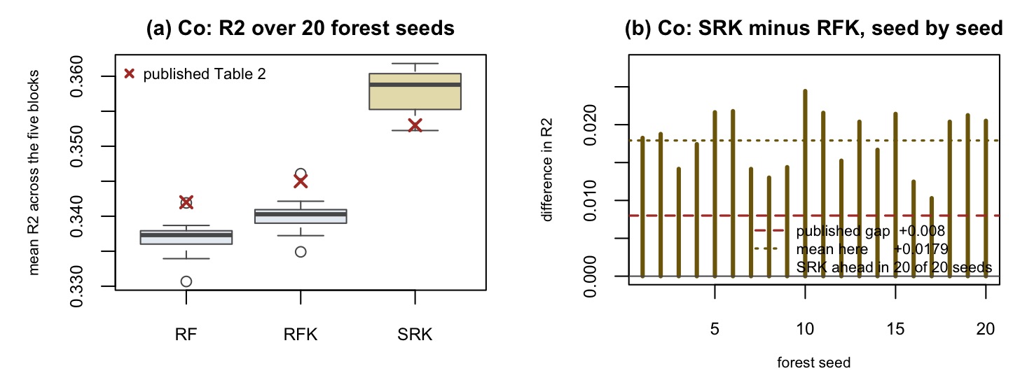
Co: SRK beats RFK on R2 in 20 of 20 seeds (mean dR2 = +0.0179, range +0.0103 to +0.0244)
Co: seed-to-seed sd of R2 is 0.0030 (SRK), the published SRK-RFK gap is 0.008
50-seed-stability took 85.2 s
== 60 Parameter sensitivity =============================
Co: best R2 0.365 at 12 km / SD 0.3; baseline 0.359
Co: 30 of 30 cells stay within +/-5% of the baseline on both metrics
60-sensitivity took 56.0 s
==================================================================
Finished in 150.4 s
Outputs: results/ tables/ figs/ data/3.2 Core Analytical Steps
Three distributions, one covariate, and where SRK's margin comes from
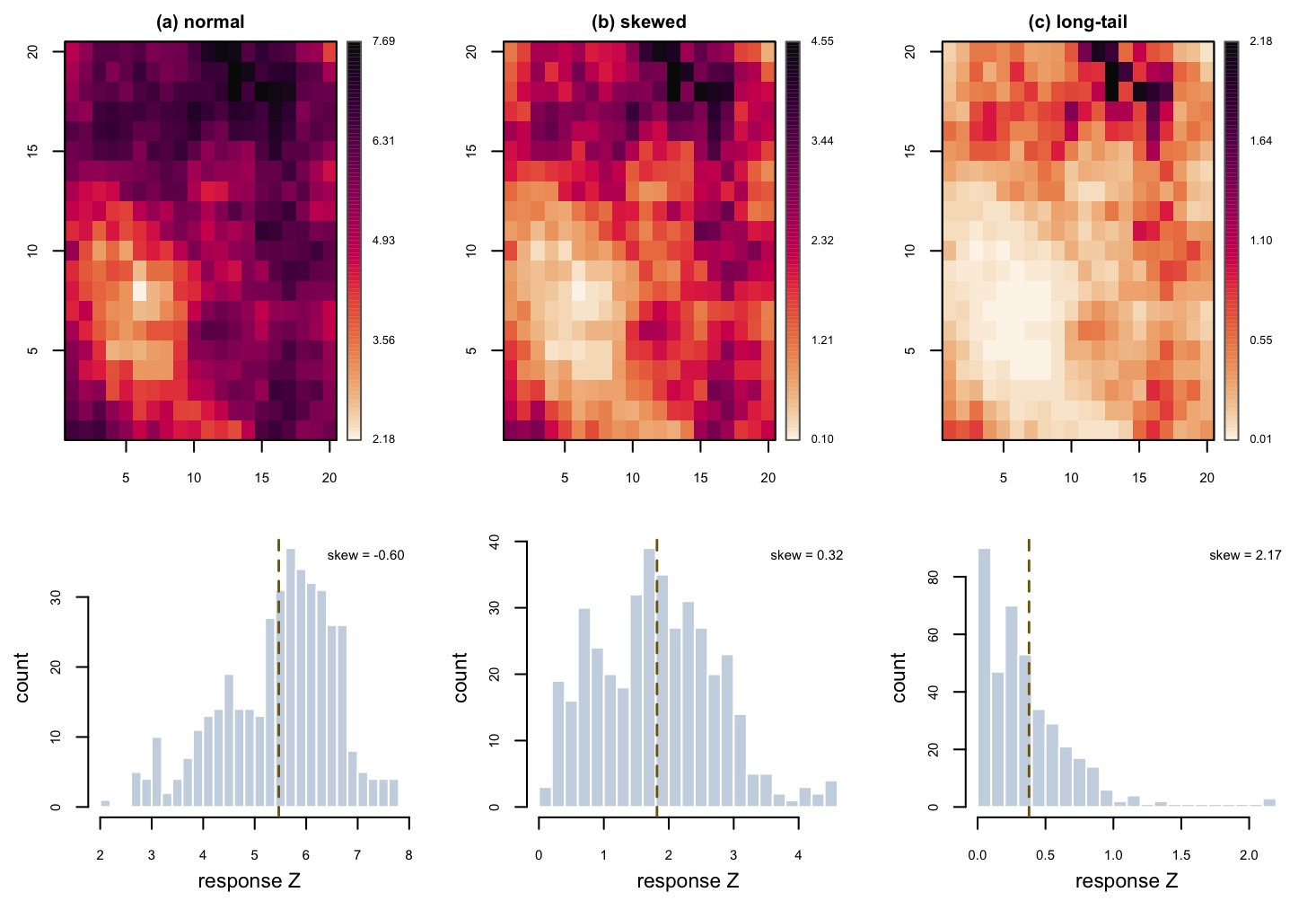
The paper's simulation is a controlled test of one claim: SRK's advantage over ordinary kriging should grow as the response departs from Gaussian. A spherical field on a 20 × 20 grid is the response; a second field, mixed 85/15 with the first, is the covariate; both are then pushed through a cube and an exponential to make a skewed and a long-tailed version. Seed 42, a 70/30 split, and the two models are scored on the held-out 120 cells.
set.seed(SEED)                                     # 42, as in the released script
xy <- expand.grid(x = seq_len(SIM_SIDE), y = seq_len(SIM_SIDE))
sp::gridded(xy) <- ~x + y

sim_field <- function(range) {
  g <- gstat::gstat(formula = z ~ 1, dummy = TRUE, beta = 0,
                    model = gstat::vgm(psill = 1, model = "Sph", range = range),
                    nmax = 20)
  stats::predict(g, newdata = xy, nsim = 1)@data$sim1
}
y_raw     <- sim_field(SIM_RANGE_Y)                # range 10
noise_raw <- sim_field(SIM_RANGE_X)                # range  8

x_raw  <- SIM_MIX * y_raw + (1 - SIM_MIX) * noise_raw   # cor(X, Y) = 0.98
y_base <- y_raw + SIM_SHIFT                             # keep the transforms positive
x_base <- x_raw + SIM_SHIFT

scenarios <- list(
  normal      = list(Y = y_base,             X = x_base),
  skewed      = list(Y = y_base^3 / 100,     X = x_base^3 / 100),
  `long-tail` = list(Y = exp(y_base) / 1000, X = exp(x_base) / 1000))
The scales here are grid cells, not metres — SV_SCALES_SIM is
1 … 10 — and the SD filter is switched off, because a single covariate
cannot be compared against anything. That matches the authors' simulation code,
which keeps its one singularity column unconditionally.
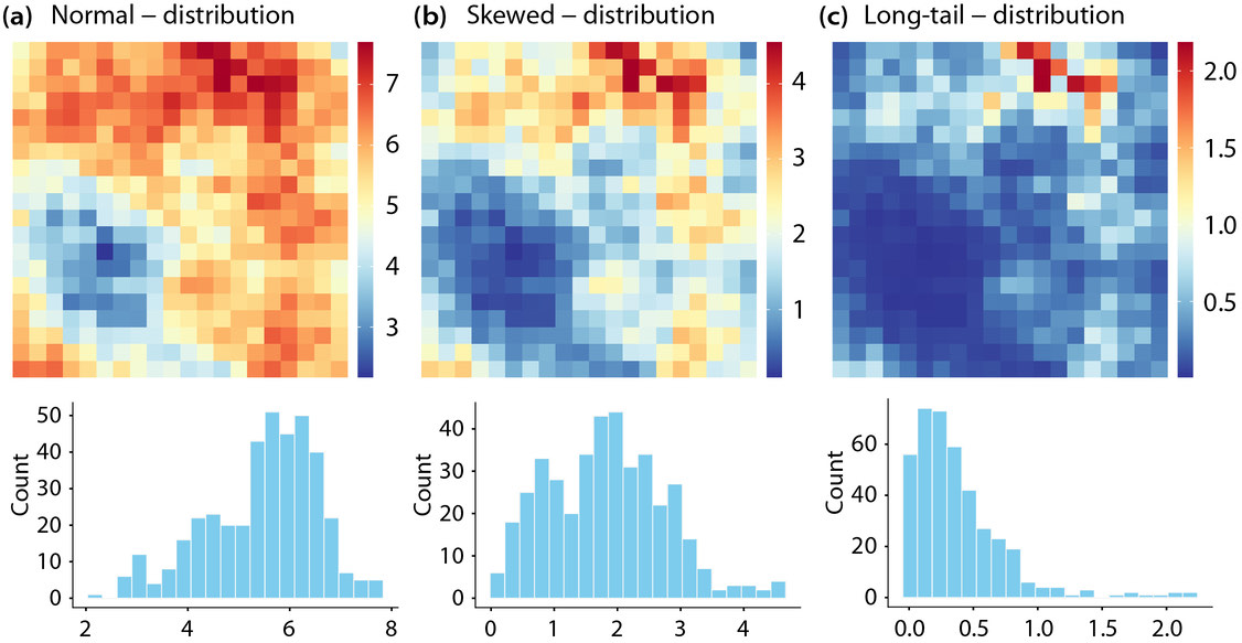
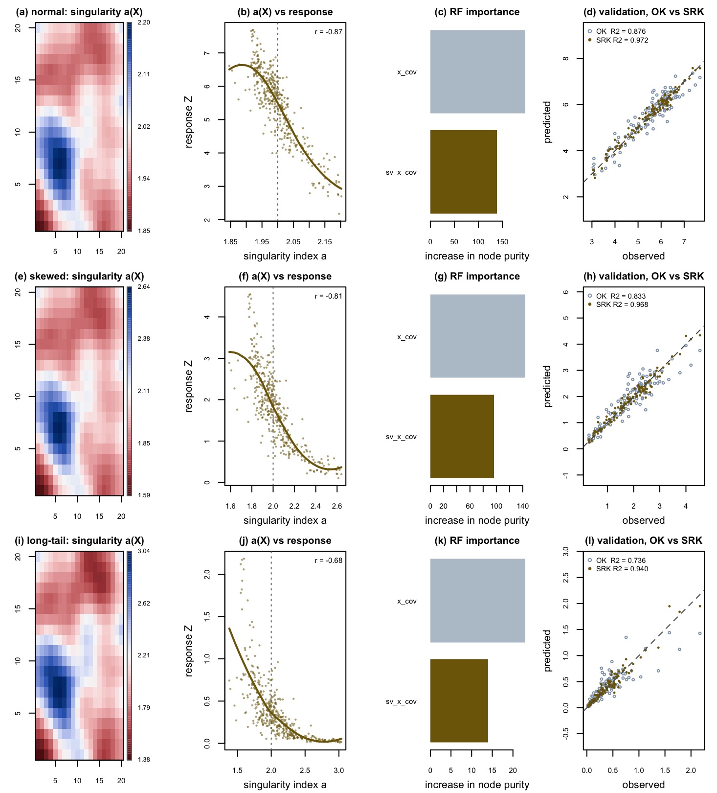
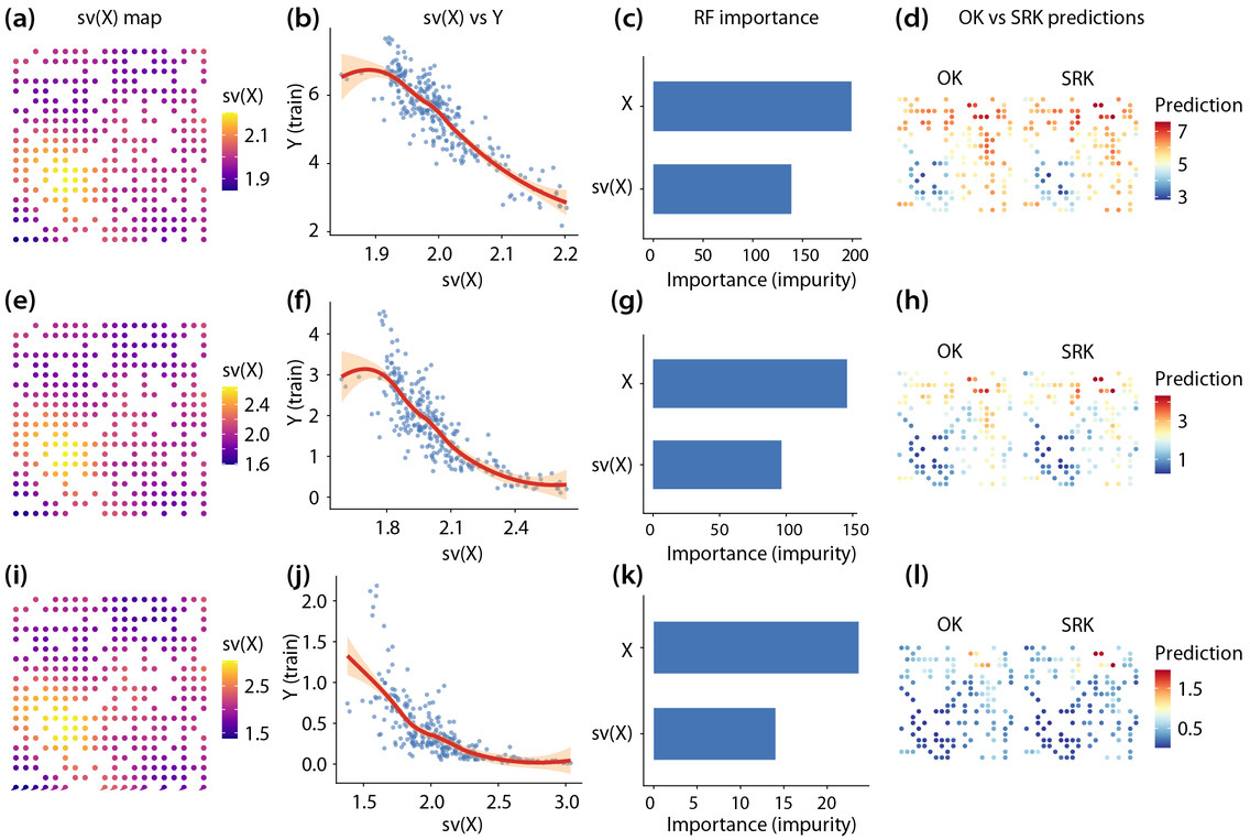
| Simulated field | R2 | RMSE | MAE | ||||||
|---|---|---|---|---|---|---|---|---|---|
| OK | SRK | paper SRK | OK | SRK | paper SRK | OK | SRK | paper SRK | |
| Normal | 0.876 | 0.972 | 0.972 | 0.361 | 0.171 | 0.172 | 0.283 | 0.137 | 0.137 |
| Skewed | 0.833 | 0.968 | 0.966 | 0.361 | 0.158 | 0.162 | 0.265 | 0.117 | 0.120 |
| Long-tail | 0.736 | 0.940 | 0.940 | 0.178 | 0.085 | 0.085 | 0.107 | 0.056 | 0.056 |
results/simulation-vs-paper.csv — the paper's
Table 1, reproduced. The three OK rows match the published values to every
printed digit. Two of the three SRK rows do too; the skewed row lands 0.002 high
in R2, which is the random forest's seed, not a difference in
method — see step 5.
The gain over ordinary kriging is 0.096 in R2 on the
near-normal field, 0.135 on the skewed one and 0.205 on the long-tailed one —
monotonically increasing, which is the paper's central simulation claim and is
asserted as a test in tests/test-02. Note also what the
simulation does not establish: the covariate here correlates 0.98 with
the response. Real covariates do not, and the case study below is where the
margin gets realistic.
Screen the covariates against the response
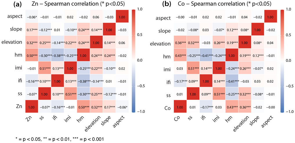
The lithology polygons have already been reduced to proximity variables by Eq. 14 — 1 inside the unit, falling linearly to 0 across a 10 km buffer. What remains is the paper's Sec. 3.2.1 screen: keep only covariates with a significant monotonic relation to the element.
sc <- do.call(rbind, lapply(CANDIDATE_XVARS, function(xv) {
  ct <- suppressWarnings(stats::cor.test(d[[yvar]], d[[xv]], method = "spearman"))
  data.frame(element = elem, covariate = xv,
             rho = unname(ct$estimate), p = ct$p.value,
             significant = ct$p.value < 0.05,
             used_by_paper = xv %in% cfg$xvars)
}))| Covariate | Spearman ρ | p | Screen | Used by the paper |
|---|---|---|---|---|
hm haematite proximity | +0.431 | 2e−46 | kept | yes |
elevation | +0.360 | 7e−32 | kept | yes |
ifi felsic intrusive proximity | −0.173 | 4e−08 | kept | yes |
imi mafic intrusive proximity | +0.031 | 0.330 | dropped | no |
slope | −0.021 | 0.508 | dropped | no |
ss sedimentary proximity | +0.005 | 0.868 | dropped | no |
aspect | −0.001 | 0.972 | dropped | no |
results/covariate-screening.csv — the screen returns
exactly the covariate set the paper reports for cobalt: IFI, HM and
elevation, with the other four dropped. This is worth stating in a manuscript:
the published covariate list is not assumed, it falls out of the data. The
separation is wide — the three kept covariates clear p < 1e−7,
the four dropped ones sit above p = 0.3.
| Element | n | mean | median | max | sd | CV | skewness |
|---|---|---|---|---|---|---|---|
| Co (ppm) | 998 | 13.30 | 8.94 | 112.2 | 13.21 | 0.994 | 2.58 |
results/response-summary.csv — the sample count matches
the article exactly. The response is strongly right-skewed (2.58) with a
coefficient of variation near 1, which is the condition the simulation says
favours SRK.
Build the singularity features, then throw one away
For each retained covariate, the intensity is measured in ten square windows of half-width 2 km to 20 km, and α is the slope of log intensity on log scale plus two. The reference points are the sample locations; the evaluation points are the same locations here, but the same call would evaluate the index on a prediction grid without changing anything.
for (xv in cfg$xvars) {
  C <- srk_intensity(d$x, d$y, d[[xv]], d$x, d$y, SV_SCALES,
                     min_pts_per_scale = MIN_PTS_PER_SCALE)      # Eq. 2
  a <- srk_alpha(C, SV_SCALES, min_valid_scales = MIN_VALID_SCALES)  # Eq. 3-4
  a[!is.finite(a)] <- SV_NEUTRAL                                 # uniform field
  Cs[[xv]] <- C                    # cached: step 60 re-cuts the ladder from this
  sv[[paste0("sv_", xv)]] <- a
}| Feature | mean α | SD | range | % α < 2 | r with Co | SD filter |
|---|---|---|---|---|---|---|
| sv(ifi) | 7.02 | 6.77 | 0.77 – 21.97 | 28.1 | +0.219 | retained |
| sv(hm) | 5.43 | 6.18 | 1.08 – 21.95 | 43.6 | −0.227 | retained |
| sv(elevation) | 2.00 | 0.046 | 1.86 – 2.16 | 44.0 | −0.172 | dropped |
results/singularity-diagnostics.csv — the SD filter is
not a close call. The two lithology proximity variables produce indices with SD
6.18 and 6.77; elevation produces 0.046. More than two orders of magnitude
separate them, and the published 0.5 threshold sits in the empty space between.
No location needed the neutral fallback: every one of the 998 samples had at
least two usable scales.
Elevation is smooth at 2–20 km. Its mean absolute value barely changes as the window grows, so the log-log slope is almost zero and α sits on 2 — the definition's own value for a uniform field. Lithology proximity is the opposite: it is 1 inside a unit and 0 more than 10 km outside, so the window mean changes sharply with scale and α ranges over an order of magnitude. The SD filter is really a smoothness detector, and the paper's 0.5 is doing exactly the job its Sec. 2.2.1 describes. (In the article's Zn model, where slope and aspect are also covariates, they behave the same way and are dropped for the same reason — SD 0.32 and 0.21.)
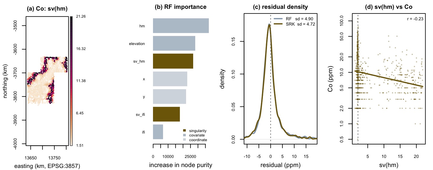
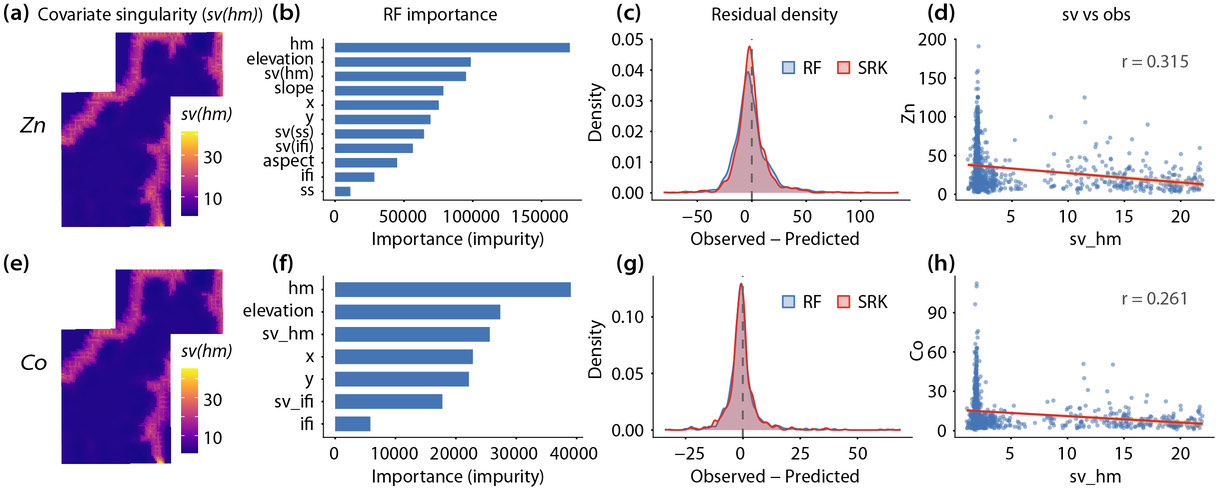
Feature importance is worth quoting directly, because it is the clearest evidence
that the singularity columns earn their place. Fitting SRK on all 998 Co samples
gives, in order: hm (23 % of total importance),
elevation (17 %), sv_hm (17 %),
x (14 %), y (14 %),
sv_ifi (11 %), ifi (4 %). Both
singularity columns outrank the raw ifi variable they were built from,
and together they carry more of the forest than the two coordinates do.
Six models, five spatial blocks, no leakage
The samples cluster heavily, so a random split would leave almost every test point ringed by its own training neighbours and would flatter every kriging-based model. The paper instead cuts the study area into 15 km squares, shuffles the squares and deals them round-robin to five folds: 120 blocks, 5 folds, whole blocks held out together.
srk_block_folds <- function(data, k = 5L, block_size = 15000, seed = 123L) {
  df <- as.data.frame(data)
  bx <- floor((df$x - min(df$x, na.rm = TRUE)) / block_size)
  by <- floor((df$y - min(df$y, na.rm = TRUE)) / block_size)
  block <- paste(bx, by, sep = "_")
  set.seed(seed)
  ub <- sample(unique(block))                       # shuffle whole blocks
  fold <- as.integer(stats::setNames(((seq_along(ub) - 1L) %% k) + 1L, ub)[block])
  attr(fold, "n_blocks") <- length(ub)
  fold
}fold <- srk_block_folds(d, CV_FOLDS, CV_BLOCK_SIZE, CV_SEED)
for (k in seq_len(CV_FOLDS)) {
tr <- d[fold != k, ]; te <- d[fold == k, ]
for (mname in names(SRK_MODELS)) { # OK IDW LM RF RFK SRK
out <- SRK_MODELS[[mname]](tr, te, yvar, cfg$xvars, sv = sv)
met <- srk_metrics(te[[yvar]], out$pred) # Eq. 11-13
...
}
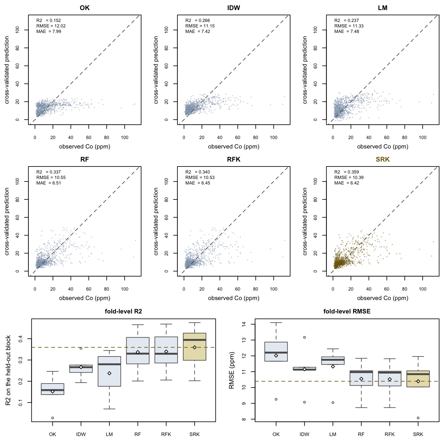
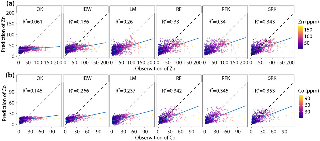
}| Model | This run | Published Table 2 | ||||
|---|---|---|---|---|---|---|
| R2 | RMSE | MAE | R2 | RMSE | MAE | |
| SRK | 0.359 | 10.39 | 6.42 | 0.353 | 10.45 | 6.47 |
| RFK | 0.340 | 10.53 | 6.45 | 0.345 | 10.48 | 6.41 |
| RF | 0.337 | 10.55 | 6.51 | 0.342 | 10.50 | 6.46 |
| IDW | 0.266 | 11.15 | 7.42 | 0.266 | 11.15 | 7.42 |
| LM | 0.237 | 11.33 | 7.48 | 0.237 | 11.33 | 7.48 |
| OK | 0.152 | 12.02 | 7.99 | 0.148 | 12.04 | 8.03 |
results/cv-summary.csv — the cobalt half of the paper's
Table 2, reproduced. IDW and LM, the two models that involve neither kriging
nor a forest, land on the published values to every printed digit — and on the
authors' own fold-level output to six decimals. Ordinary kriging is 0.004 high in
R2 because autoKrige picks a different variogram
family on two of the five folds (§3.5). The three
forest models are within the seed spread measured in step 5, and SRK is
first here as it is in the article.
Matters. Ordinary kriging explains 15 % of the cobalt variance under spatial blocking; adding covariates through a forest takes that to 36 %, and reduces RMSE by 14 % and MAE by 20 %. That is a large, robust, unambiguous effect, and it is the same conclusion the article draws.
Needs an error bar. SRK against RFK is 0.020 in R2
here, against 0.008 in the article — and the authors' own released
cv_summary_Co.csv has the two the other way round, with RFK ahead
by 0.001. Three artefacts, three answers. A gap that size cannot be read off a
single run of a model containing an unseeded random forest. That is what
step 5 is for.
Is the SRK lead real? Put an error bar on it
Three of the six models contain a random forest, and the released scripts call
ranger() without a seed. So RF, RFK and SRK produce a different number
every time the analysis is run — and the differences the article reports between
them are small. There is direct evidence of how small: the authors' own repository
ships cv_summary_Co.csv with SRK at
R2 = 0.344, behind RFK at 0.345, while the
article's Table 2 has SRK first at 0.353. Same code, same data, different run.
This step holds the folds and the data fixed and repeats the entire cross-validation over 20 forest seeds, then asks a paired question: on how many of those seeds does SRK actually finish ahead of RFK?
fold <- srk_block_folds(d, CV_FOLDS, CV_BLOCK_SIZE, CV_SEED)   # fixed once

for (s in seq_len(SEED_REPEATS)) {
  for (mname in c("RF", "RFK", "SRK")) {                       # the seeded three
    fm <- do.call(rbind, lapply(seq_len(CV_FOLDS), function(k) {
      out <- SRK_MODELS[[mname]](d[fold != k, ], d[fold == k, ],
                                 yvar, cfg$xvars, sv = sv, seed = s)
      srk_metrics(d[[yvar]][fold == k], out$pred)
    }))
    ...   # mean over the five blocks, one row per (seed, model)
  }
}
| Model | mean R2 | SD | min | max | published | authors' CSV |
|---|---|---|---|---|---|---|
| SRK | 0.3580 | 0.0030 | 0.3522 | 0.3618 | 0.353 | 0.344 |
| RFK | 0.3401 | 0.0022 | 0.3349 | 0.3461 | 0.345 | 0.345 |
| RF | 0.3369 | 0.0022 | 0.3307 | 0.3419 | 0.342 | 0.342 |
results/seed-stability-spread.csv — the seed-to-seed SD is
about 0.002–0.003 in R2 for all three models. The published RFK
value falls inside the range; the published RF value sits 0.0003 above the top of
it; the published SRK value is inside. The one number that falls clearly outside
is the authors' released CSV for SRK (0.344), which is lower than any of the
20 seeds here — see the note below.
SRK finishes ahead of RFK on 20 of 20 seeds, by +0.018 in R2 on average, with the smallest margin (+0.010) still more than three times the seed-to-seed SD. That is a stronger result than the article claims for cobalt (+0.008), and it is the kind of statement a paired design licenses and a single run does not.
The comparison that never needed an error bar is SRK against the geostatistical benchmarks: +0.21 in R2 over ordinary kriging is seventy times the seed noise. Reporting the spread separates the claim that is bulletproof from the one that had to be earned.
The authors' released SRK value of 0.344 is about five seed-SDs below the
mean this pipeline produces, so the forest seed alone does not explain it.
SRK's third step is an autoKrige call on the residuals, and the
same automap version difference that shifts ordinary kriging on two
of the five folds (§3.5) shifts SRK too. Both effects
are real, both are small compared with SRK's margin over OK, IDW and LM, and
both are worth naming rather than averaging away.
Any comparison between two models that both contain a random forest needs this. It costs one loop and it changes what you are entitled to write. If the gap between your method and the nearest benchmark is smaller than the spread across seeds, report the spread — a reviewer who re-runs your code will find it anyway.
How much do the two parameters matter?
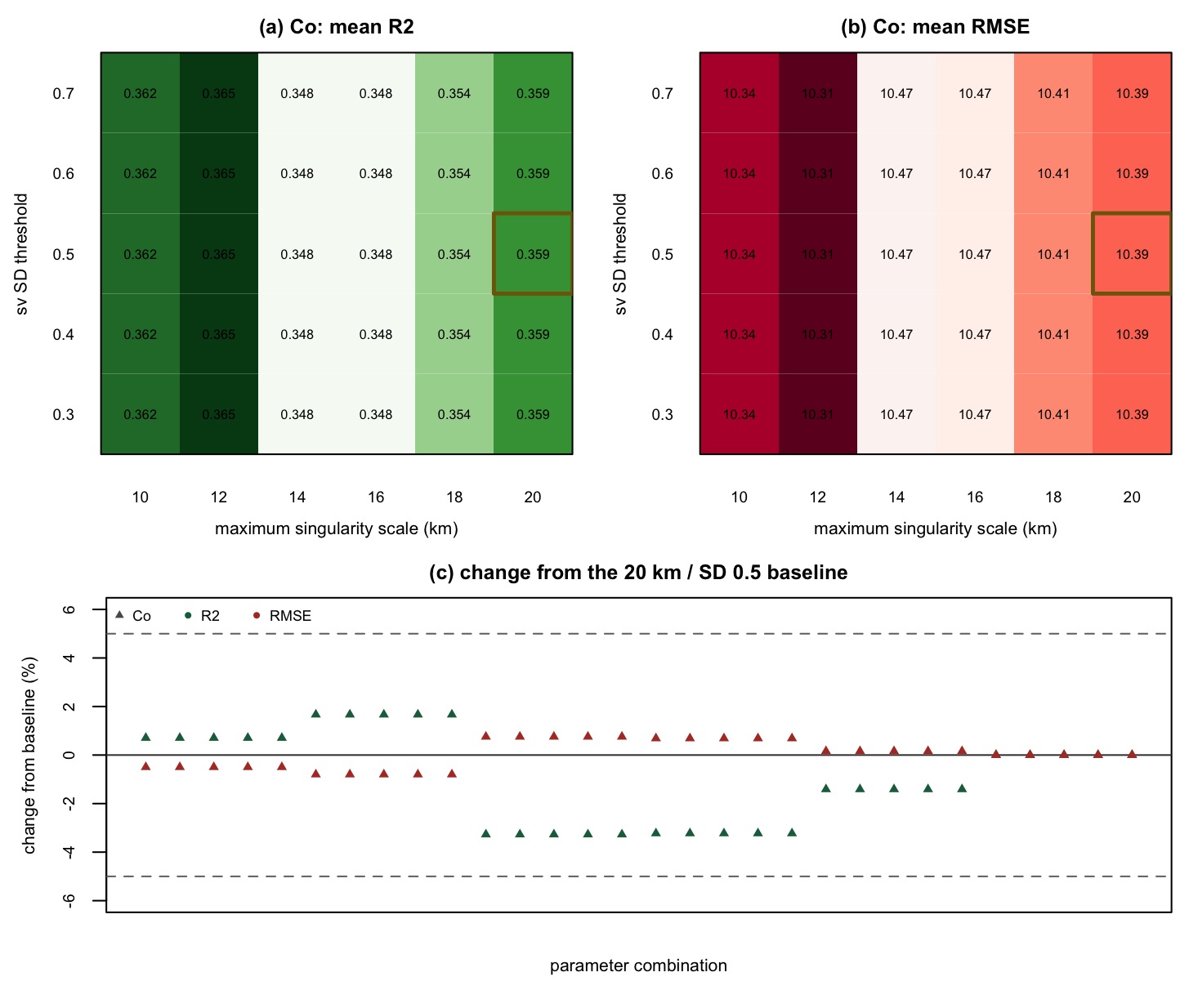
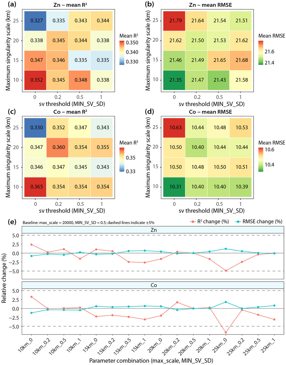
SRK has exactly two tuning choices: how far up the scale ladder the regression runs, and how flat a singularity feature may be before it is dropped. The paper varies both and reports that performance stays within roughly ±5 % of the baseline. This step re-runs the full cross-validation over a 6 × 5 grid of the two — 30 cells, 150 SRK fits.
Truncating the ladder needs no new neighbourhood search. Step 3 cached the per-scale intensity matrix, so a shorter ladder is a column subset and a re-fitted slope:
Cs <- readRDS(file.path(DERIVED, sprintf("intensity-%s.rds", elem)))

for (mx in SENS_MAX_SCALES) {              # 10, 12, 14, 16, 18, 20 km
  keep_scale <- SV_SCALES <= mx
  for (xv in cfg$xvars) {                  # re-fit Eq. 3-4 on the shorter ladder
    a <- srk_alpha(Cs[[xv]][, keep_scale, drop = FALSE], SV_SCALES[keep_scale],
                   min_valid_scales = MIN_VALID_SCALES)
    a[!is.finite(a)] <- SV_NEUTRAL
    sv[[paste0("sv_", xv)]] <- a
  }
  for (thr in SENS_THRESHOLDS) { ... }     # 0.3, 0.4, 0.5, 0.6, 0.7
}
| baseline R2 | best | at | ΔR2 range | ΔRMSE range | cells within ±5 % |
|---|---|---|---|---|---|
| 0.359 | 0.365 | 12 km / any threshold | −3.3 % to +1.7 % | −0.8 % to +0.8 % | 30 / 30 |
results/sensitivity.csv — the article's robustness claim
reproduces: every combination stays inside ±5 % of the baseline on both
metrics, and RMSE moves by less than one percent across the whole grid.
Read the heatmaps down a column rather than across: every threshold from 0.3 to 0.7 gives the identical number. That follows from step 3 — the retained features have SD 6.18 and 6.77 and the dropped one 0.046, so nothing in the 0.3–0.7 range changes which features are kept. The threshold is not tuning anything on this data; it is a switch sitting far from its own decision boundary. That is a comfortable place to be, and quite different from the CRAN package's simulated data, where the same 0.5 lands on the wrong side of the only feature there is (§1.4).
The scale ladder does move the answer, mildly and non-monotonically: cobalt peaks at 12 km (0.365) against 0.359 at the published 20 km. That is a 1.7 % gain — the same order as the seed noise in step 5, so the location of the optimum is not sharply identified either. The article's own sensitivity analysis reaches the same verdict from the other direction: nothing in the grid is far from anything else.
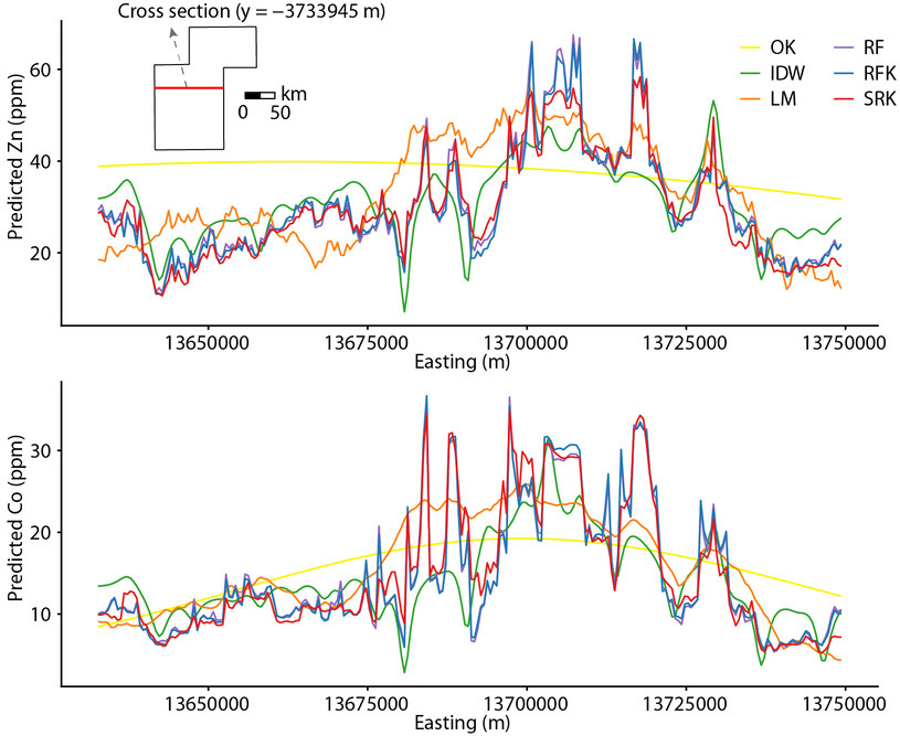
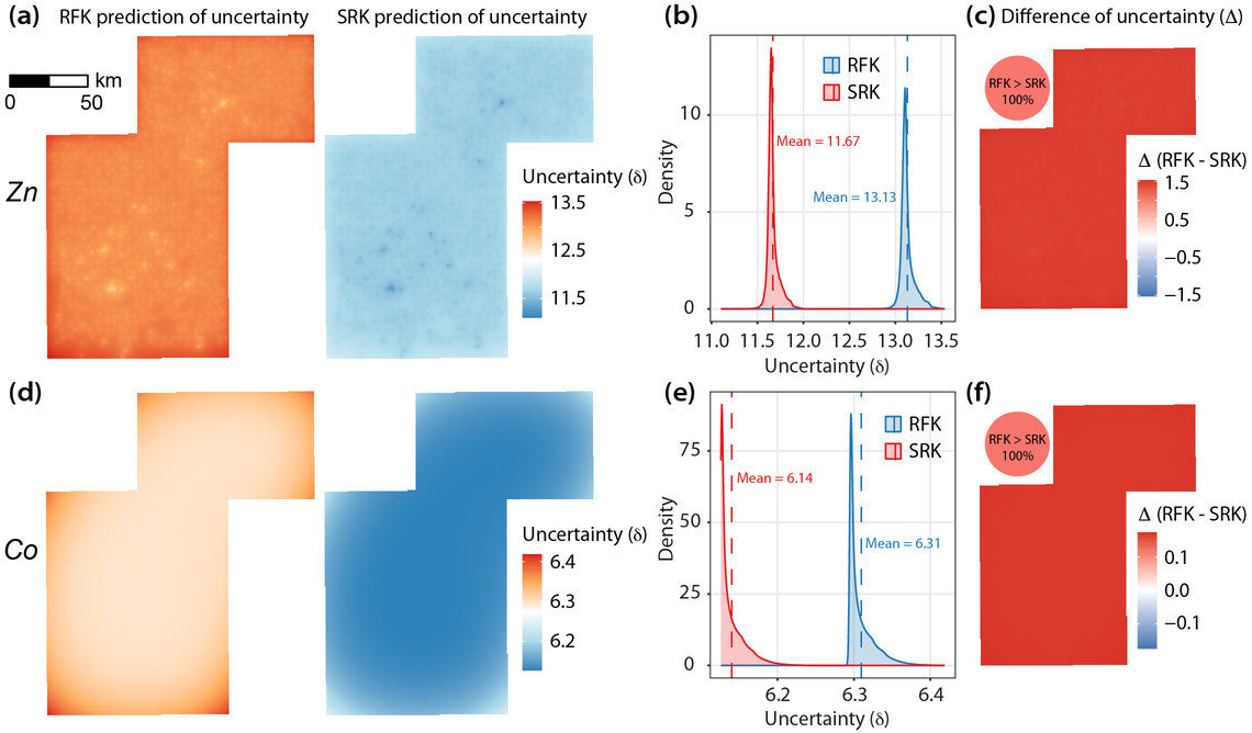
3.3 What the Article Shows Beyond Cross-Validation
The figure at the top of this page and the two below are the part of the article this
pipeline deliberately does not regenerate. They all need the 97,234-cell, 500 m
prediction grid — an 8.1 MB covariate table on which the singularity indices, the
forest trend and the kriging system must all be evaluated. Adding it is not conceptually
different from what step 4 already does: srk_run() takes a
pred_data-shaped test frame, and R/30-singularity.R already
evaluates α at arbitrary locations. It is a change of scale, not of method — and
the point of a tutorial that stops at cross-validation is that every number on this page
can be checked in two and a half minutes on a laptop.
Download raw data/grid_linear.csv from the authors' repository into
data/, evaluate srk_intensity() with the sample points as
reference and the grid as evaluation set (the function is chunked for exactly this),
then call srk_run() once with the grid as test. Budget most
of the time for the 97,234 × 998 neighbourhood search and for the
kriging system; the authors precompute the former into
sv_precomp_*.rda for the same reason.
3.4 Reading the Results Together
Six steps produce one argument, and it is worth stating in the order a reader will want it.
- The mechanism is real and it is visible. Singularity indices built from
lithology proximity vary over an order of magnitude, correlate with cobalt at
r = +0.22 and −0.23, and the forest ranks sv(hm) third of seven
features — above both coordinates, and above the
ificovariate that sv(ifi) was derived from. - Under controlled conditions the gain is large and behaves as predicted. On the simulation, +0.096, +0.135 and +0.205 in R2 over ordinary kriging as the response goes from near-normal to long-tailed. Monotone, as the paper claims.
- On real data the gain over kriging is large; over a forest it is small but consistent. SRK beats OK by +0.21 in R2 and cuts RMSE by 14 %. Against RFK the margin is +0.018 — small, but positive on every one of 20 forest seeds.
- The residual really does get easier to krige. On the full-sample fit, residual SD falls from 4.90 to 4.72 ppm when the two singularity columns are added — which is the mechanism the article's Fig. 11 turns into lower kriging variance.
- Nothing here is delicate. Thirty parameter combinations stay within ±5 % of the baseline, and the SD threshold is nowhere near a decision boundary. The quantity that does need care is the SRK–RFK margin, and step 5 measures it rather than asserting it.
| Claim | Where it is tested | Verdict from this run |
|---|---|---|
| SRK > OK under non-Gaussianity, margin growing with skew | Step 1, Table 1 | reproduced to three decimals |
| The published covariate set follows from the data | Step 2, Fig. 5 | reproduced exactly |
| The SD filter separates informative from flat features | Step 3, Fig. 6 | reproduced; the separation is two orders of magnitude |
| SRK > OK, IDW and LM under spatial blocking | Step 4, Table 2 | reproduced, large margin |
| SRK > RFK | Steps 4–5 | holds on 20/20 forest seeds, by more than the article claims |
| Insensitivity to the two parameters | Step 6, Fig. 7 | reproduced; 30/30 cells inside ±5 % |
| Lower prediction uncertainty than RFK | article Fig. 11 | out of scope here; the residual-SD reduction that drives it is reproduced |
3.5 Validation
Rscript run-all.R test runs two suites in about eight seconds.
test-01 checks the implementation against the definitions;
test-02 checks the outputs against the published article and against
the authors' own released fold-level numbers.
== test-01  Method properties =============================================
   intensity equals the mean |X| inside the square window     pass
   vectorised singularity matches the authors' loop           pass
   a uniform field gives alpha = 2 everywhere                 pass
   alpha equals the fitted log-log slope plus two             pass
   a field growing away from a source is depleted (alpha > 2) pass
   SD filter keeps the varying feature and drops the flat one pass
   SRK prediction equals trend plus kriged residual (Eq. 9)   pass
   a block is never split across folds                        pass
   singularity is computed from covariates, not the response  pass
   ...
   18/18 checks passed

== test-02  Reproduction of the published results ========================
   Co sample count is the paper's 998                         pass
   the response is right-skewed, as Sec. 4.1 describes        pass
   Spearman screen reproduces the published Co covariates     pass
   imi is screened out, as in Sec. 4.2                        pass
   lithology singularity SD is above the 0.5 threshold        pass
   terrain singularity SD is below it                         pass
   sv(hm) is among the three most important SRK features      pass
   simulated OK matches Table 1 to 0.001                      pass
   simulated SRK matches Table 1 to 0.005 (forest seed)       pass
   the SRK margin widens as the distribution departs from normal pass
   all 10 deterministic fold results were found               pass
   IDW and LM reproduce the authors' fold R2 to 1e-6          pass
   IDW and LM reproduce the authors' fold RMSE to 1e-5        pass
   Co: ordinary kriging is last, as in Table 2                pass
   Co keeps SRK ahead of RFK on every forest seed             pass
   the seed-to-seed spread is smaller than the SRK-RFK gap    pass
   every parameter combination stays within +/-5% of the baseline pass
   ...
24/24 checks passedtest-02 embeds the authors' released fold-level results for the two
benchmarks that contain no random forest — IDW and LM — and requires this pipeline
to match all ten of them to 1e−6. Those two models are pure functions of the
fold assignment and the data, so matching them proves that the 998 samples, the 120
blocks and the five folds built here are the same objects the published analysis
used. Everything else in the comparison then rests on something firmer than "the
numbers look similar".
Ordinary kriging matches the authors' released fold-level output exactly on folds
1, 4 and 5, and differs on folds 2 and 3
(R2 0.247 against 0.241, and 0.189 against 0.160). That moves
the OK mean from their 0.145 to 0.152 here, against 0.148 in the article.
automap::autoKrige chooses the residual variogram family automatically,
and on those two folds the choice differs between package versions. The same
mechanism nudges SRK, whose third step is also an autoKrige call. Both
are recorded in env/requirements.md rather than papered over; neither is
large enough to change any ordering in Table 2.
4 Adaptation, Writing & Reproducibility
4.1 Port to Your Domain
SRK needs a point response, covariates observable everywhere, and projected
coordinates. Nothing about it is specific to geochemistry — soil properties, air
pollution, groundwater chemistry, biomass and disease incidence all have the shape it
wants. Four edits to config/project-config.R and the pipeline runs on your
data.
| # | Edit | How to choose |
|---|---|---|
| 1 | DATA_SOURCE <- "local", then one CSV per response in data/ |
Columns x, y, the response, one per covariate. Use a
projected CRS in metres — UTM or an equal-area projection, not Web Mercator
(§2.4). |
| 2 | ELEMENTS and CANDIDATE_XVARS |
List every covariate you have; step 20 screens them and tells you which survive at p < 0.05. Start from that set rather than deciding in advance. |
| 3 | SV_SCALES |
The single most important choice. The ladder should span the scales your
covariate actually varies over, and every scale needs
MIN_PTS_PER_SCALE samples inside the window — so the smallest
scale is bounded from below by your sampling density. A practical rule: start
the ladder at roughly twice the median nearest-neighbour distance and end it
near a fifth of the study-area extent. |
| 4 | CV_BLOCK_SIZE |
Large enough that a held-out block is genuinely independent of its training neighbours — of the order of the variogram range, not smaller. Too small and you are back to a random split; too large and folds become unbalanced. |
Run steps 20 and 30 and look at results/singularity-diagnostics.csv
before anything else. If every sv_sd comes back near zero, your
covariates are smooth at the scales you chose and SRK has nothing to add over plain
regression kriging — either widen the ladder or find a covariate with genuine local
structure. If n_neutral is large, the ladder is finer than your
sampling design supports and the indices are being imputed rather than estimated.
Both failures are silent in the accuracy table and obvious in that one file.
Design decisions worth making deliberately
- Coordinates in the forest or not.
RF_USE_COORDS = TRUEreproduces the published case study;FALSEfollows Eq. 5. Leaving them in lets the forest learn location directly, which competes with the job the kriging step is there to do — for cobalt the two coordinates take 28 % of the forest's total importance between them. If your interest is in why the response varies rather than only in prediction accuracy, run it both ways and report both. - Reference set for the index. Here the reference points are the sample locations, so the index inherits the sampling design. If your covariate exists as a raster, evaluating the intensity on the raster instead removes that dependence entirely and is closer to the theory in Eq. 1–2. That is a real modelling choice, not a detail.
- Anisotropy. Both the article and this pipeline krige isotropically. In a
structurally controlled setting — a fault trend, a prevailing wind, a river network —
fitting an anisotropic variogram to the residual is the obvious next thing to try;
automapwill not do it for you. - Back-transformation. The response is modelled on its raw ppm scale, not logged, even though it is strongly right-skewed. If you log a skewed response, remember that exponentiating the prediction is biased low, and say what correction you applied.
4.2 Write the Paper
The article's own structure is the template, and this pipeline produces a table or a figure for every part of it.
| Manuscript section | What to report | From |
|---|---|---|
| Data and preprocessing | sample counts, response summary, how categorical covariates became continuous | results/response-summary.csv, data/provenance.md |
| Variable selection | the Spearman screen, with ρ and p for every candidate, including the ones dropped | tables/table-covariate-screening.tex |
| Singularity features | the scale ladder, the minimum counts, the SD filter, and what it kept — with the SDs, so the threshold is visibly not arbitrary | tables/table-singularity-features.tex |
| Model and validation design | 500 trees, autoKrige, isotropy, block size, fold count, block count | §3.2 Step 4 |
| Accuracy | all six models, all three metrics, differences quoted against your method | tables/table-model-comparison-*.tex |
| Robustness | the parameter grid and the seed spread | tables/table-seed-stability.tex, results/sensitivity.csv |
| Interpretation | feature importance — the sentence that says the singularity column outranks the covariate it came from is the one reviewers remember | results/rf-importance.csv |
- "Singularity indices were computed from covariates rather than from the response, so they are defined at unsampled locations and inside held-out blocks." — this is the methodological point, and it is what distinguishes SRK from a feature that would leak.
- "Cross-validated differences among the forest-based models were compared against the spread over N random-forest seeds." — with the number. It costs a loop and it forecloses the most obvious referee objection.
- "Coordinates were / were not included in the trend model." — state it. Two papers running "the same" model with different answers here are not running the same model.
4.3 Final Reproducibility Package
| Artefact | Contents |
|---|---|
srk-code-and-data.zip (about 176 KB) |
run-all.R, R/, config/,
tests/, plus results/ and tables/ so
every number on this page can be read without running anything |
R/02-srk-core.R |
the method and the five benchmarks in one file, with the paper's equation
numbers in the comments and every departure marked
DEPARTURE |
tests/ |
18 method-property checks and 24 reproduction checks, including a literal
transcription of the authors' singularity_safe() loop to verify
the vectorised port |
env/requirements.md |
package list, per-step runtimes, and the one known version sensitivity |
data/provenance.md |
where the samples come from, what the coordinates are, and what is deliberately not downloaded |
figs/ |
every figure as 196 dpi PNG and as vector PDF |
The data are not in the zip by design. They belong to the GSWA geochemistry database
and Geoscience Australia, they are already published by the article's authors, and a
tutorial should point at the source rather than fork it. R/20-case-data.R
fetches the one table it needs in under a second and records where it came from.
unzip srk-code-and-data.zip && cd SRK
Rscript -e 'install.packages(c("sp","gstat","automap","ranger"))'
Rscript run-all.R          # about 150 s
Rscript run-all.R test     # 18 + 24 checks
Every figure on this page tagged Demo run, and every number quoted from
results/, comes out of that. Figures tagged Published reference
are images from the open-access article
(CC BY) and are
reproduced here with attribution.
Sources
- Ren K, Song Y, Chen M, Yu Q (2026). A singularity regression kriging for spatial prediction. GIScience & Remote Sensing 63(1):2690341. doi:10.1080/15481603.2026.2690341 · local PDF
- Authors' code and data: github.com/renkaigis/Singularity_Regression_Kriging · Figshare
- Cheng Q (2017). Singularity analysis of geo-anomalies — the source of the scaling relation in Eq. 1–4.
- Breiman L (2001). Random forests. Machine Learning 45:5–32.
- Hiemstra P et al. (2009).
automap; Pebesma E (2004).gstat; Wright M & Ziegler A (2017).ranger. - GSWA Geochemistry database (DMIRS-047); Geoscience Australia, Surface Geology of Australia (2012) and Digital Elevation Model (2015).