Reproducible models · Tutorial 4 of 13
Reproducing Local Pathways of Association
A complete walkthrough of the LPA model — path analysis made local, so that the coefficient linking climate to vegetation is allowed to differ between the northern Qiangtang and the southeastern gorges instead of being averaged into one number for the whole Tibetan Plateau. From Ripley's K to the published table, on the published case.
To cite the LPA model and its codes in publications, please use:
Hu J, Qu R, Song Y, Wu P (2025). Local pathways of association. International Journal of Applied Earth Observation and Geoinformation 139:104531. doi · PDFopen access
Rosseel Y (2012). lavaan: an R package for structural equation modeling. Journal of Statistical Software 48(2):1–36. doi · CRAN
R/ pipeline scripts · config/project-config.R · data/lpa-tibetan-plateau.csv (1,801 sampling locations, the published case, carrying both the observed variables and the authors' own output) · tests/ · run-all.R — unzip and run Rscript run-all.R test from the LPA/ folder root.
1 Method Overview & Reproduction Scope
1.1 Core Idea
Path analysis answers a question correlation cannot: not whether climate and vegetation move together, but how much of that movement runs through soil. A structural equation model estimates the strength of each arrow in a hypothesised causal diagram, and reports it as a path coefficient λ.
Over a study area the size of the Tibetan Plateau, one λ per arrow is a claim that the same causal chain operates the same way at every location — from the monsoon-fed southeastern gorges to the cold desert of the northwest, 3,000 km away. LPA drops that assumption. It fits the same structural equation model separately inside a neighbourhood around every location, so each arrow becomes a surface rather than a scalar, and the variation of that surface becomes the result.
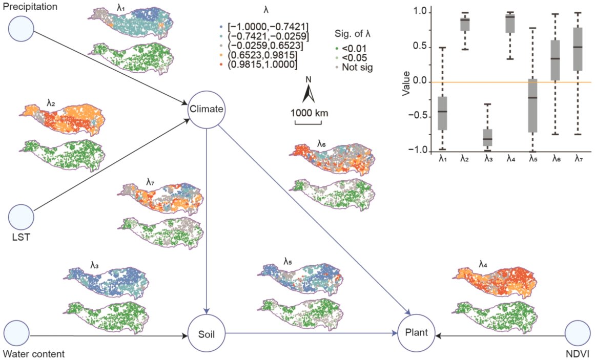
- Research problem: path coefficients estimated globally absorb regional differences into an average, and the average can be an artefact — the paper's own λ for climate on soil runs from −0.969 to 0.997 across space while the global model reports a single 0.677.
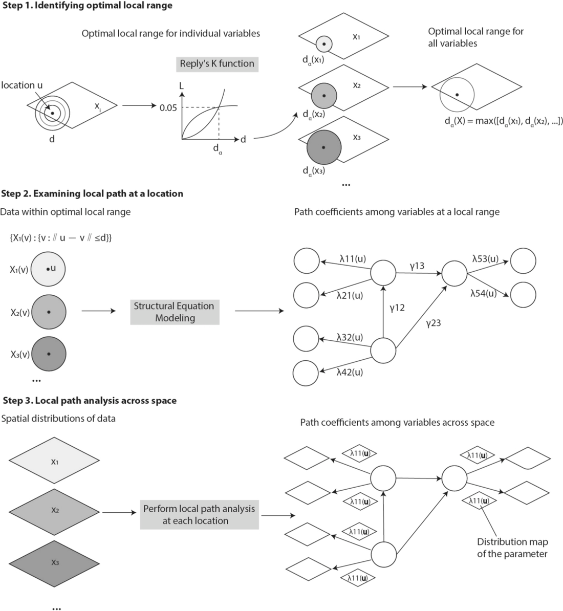
- One-line contribution: LPA determines a local range from the data with Ripley's K, estimates the structural equation model inside that range at every location, and maps the resulting path coefficients and their significance.
- Why it matters: a global coefficient tells you a relationship exists somewhere; a local one tells you where, and where it reverses. On this case, three of the seven pathways are significant at fewer than 71 % of locations, which a single starred coefficient in a conventional SEM table would never reveal.
1.2 Method Logic
ropt = 705.29 km herelavaan::sem() on ~596 neighbours1,801 fits → 7 maps
Key concepts and equations
- Ripley's K counts neighbours at a distance. For a distance r, K(r) is the expected
number of further points within r of a typical point, scaled by the study area A and the
point count n:
K(r) = (A/n²) Σi Σj≠i I(dij ≤ r)Under complete spatial randomness K(r) = πr². Anything above that is clustering.
- Besag's L makes it readable, and its peak is the local range. The square-root
transform turns the quadratic expectation into a straight line at zero, so the curve can be
read directly:
L(r) = √(K(r)/π) − r ropt = arg maxr L(r)L(r) > 0 means the points are more clustered than random at that distance, and the distance at which L peaks is the scale at which spatial interaction is strongest. That distance becomes the radius of every local model.
- The local structural equation model. At location u, only the observations within
da(Xi) of u enter the fit:
{Xi(v) : ‖u − v‖ ≤ da(Xi)}Inside that window the usual path equations apply, with every coefficient now carrying the location as an argument:X2 = λ21(u) X1 + ε1 X3 = λ32(u) X2 + λ31(u) X1 + ε2Estimation is ordinary maximum likelihood, λ̂ = arg minλ Σ(yi − ŷi)². Nothing about the estimator is new — the locality lives entirely in which rows are passed to it.
- Across space, λ becomes a function of position. Repeating the fit at u1 … un yields λij(u) = f(u), a surface that can be mapped, summarised and significance-tested like any other spatial variable.
The estimated range of 705 km puts a median of 596 of the 1,801 locations inside every
neighbourhood — a third of the study area per fit. Neighbouring models therefore share most of
their data, which is what makes the resulting surfaces smooth, and also what stops any single
map cell from being an independent observation. The radius is the method's main free choice,
and R/50-radius-sensitivity.R exists to keep that choice visible.
1.3 Reproduction Scope
This page reproduces two different things, and keeping them apart is the point.
| What | Against | Result |
|---|---|---|
| Table 2 — all seven pathways, mean [min, max] and share significant | the authors' published output file | exact, 28 of 28 printed figures |
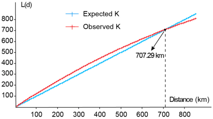
| Fig. 4 — the optimal local range | the published 707.29 km | 705.29 km, a difference of 0.3 % |
| Fig. 5 — the seven coefficient maps, their significance maps and the boxplot | the published output file | redrawn, same class breaks |
| The authors' violin plot | the attached result with LSEM.R |
redrawn as written |
| The λ surfaces themselves, refitted from the observed variables | the published λ, location by location | partial — see §3.3 Step 3 |
What this page reproduces, and against what. The published Table 2 values are matched exactly; the optimal local range differs by 0.3 % because it is re-estimated rather than read off.
The article states the LPA model but not the structural equation specification behind its numbers, and the code released with it draws the violin plot rather than estimating the pathways. The specification used here is therefore inferred from the output file (§2.4). It recovers the sign and the spatial pattern of the published surfaces; it does not recover the individual estimates. Everything on this page that depends on that inference is labelled as a refit, and everything labelled exact depends only on the authors' own numbers.
How to use this page
Read §2 to get the pipeline running, then §3.2 to confirm it reproduces the published table before trusting anything else it prints. §3.3 walks the method one step at a time, each with the code, the console output it produces and the figure it draws. §4 is for porting the model to another study area.
2 Setup, Structure & Data Contract
2.1 Environment & Dependencies
Two packages carry the method: spatstat.explore for Ripley's K and
lavaan for the structural equation model. Neither is called through a wrapper — LPA
is an arrangement of standard tools rather than a new estimator, which is why it ports easily to
other disciplines.
# The two that do the work
install.packages(c("lavaan", "spatstat.explore", "spatstat.geom"))

# Figures
install.packages(c("ggplot2", "patchwork"))| Package | Role in the pipeline | Version |
|---|---|---|
spatstat.explore, spatstat.geom |
Kest() with edge correction, and the observation window it is corrected against (Step 1) | 3.8.1 / 3.8.2 |
lavaan |
sem() and standardizedSolution() at every location (Steps 2–3) | 0.7.2 |
ggplot2 | every figure | 4.0.3 |
patchwork | the two-panel K and L figure only | 1.3.2 |
| base R | distances, neighbourhoods, the convex hull outline, the summaries | 4.6.0 |
Package roles and the versions the pipeline was run with. Only spatstat and lavaan do analytical work; the rest draw figures.
The pipeline reads a plain CSV of coordinates and variables, so sf,
terra and GDAL are not needed. Distances are Euclidean on an equirectangular
plane, which is the convention that reproduces the published range; if your study area spans
more latitude than this one, project the coordinates properly before Step 1 and set
PROJECTION <- "degrees" so the pipeline leaves them alone.
2.2 Project Structure & Configuration
LPA/
├── run-all.R                        one command runs everything
├── config/project-config.R          the only file you edit to port the model
├── R/
│   ├── 00-config.R  01-helpers.R    paths, logging, neighbourhoods, the local fit
│   ├── 10-prepare-data.R            read, project, describe
│   ├── 20-optimal-range.R           Ripley's K -> r_opt          (Step 1)
│   ├── 30-local-sem.R               one SEM per location         (Steps 2-3)
│   ├── 40-reproduce-published.R     rebuild Table 2, then test the refit
│   ├── 50-radius-sensitivity.R      how much the radius decides the answer
│   ├── 90-tables.R                  LaTeX tables
│   └── p01..p04                     figures
├── data/
│   ├── lpa-tibetan-plateau.csv      1,801 locations, the published case
│   ├── LSEM_out.xlsx                the same data as the authors distributed it
│   ├── original-violin-plot.R       the authors' own plotting script, unedited
│   └── derived/                     points.rds, r-opt.rds, neighbour counts
├── results/  tables/  figs/         everything the pipeline writes
├── tests/                           31 assertions against the paper, 10 on the method
├── env/                             session info, package versions
└── assets/                          reference figures from the article
Every choice the method makes is a named constant in one file. Porting the model to another
study area means editing config/project-config.R and nothing else.
# -- Input ---------------------------------------------------------------
INPUT_FILE <- "data/lpa-tibetan-plateau.csv"
COORD_X    <- "x"          # longitude, decimal degrees
COORD_Y    <- "y"          # latitude,  decimal degrees

# -- The optimal local range ---------------------------------------------
# Edge correction matters more than anything else here: with no correction
# the L curve peaks at roughly half the published distance.
K_CORRECTION <- "border"       # "border", "isotropic" or "none"
K_WINDOW     <- "rectangle"    # bounding box, or "hull"
K_R_MAX      <- 1200           # km, upper end of the search grid
MIN_LOCAL_N  <- 60             # a fit needs enough neighbours to be worth trusting

RADIUS_OVERRIDE    <- NULL     # set a number to force a radius
RADIUS_SENSITIVITY <- c(400, 500, 600, 705.29, 800, 900)

# -- The structural equation model ---------------------------------------
SEM_MODEL <- '
  Plant   =~ EVI + NDVI
  Climate =~ T + LST + P
  Soil    =~ PH + watercontent

  Soil  ~ Climate
  Plant ~ Climate + Soil
'

# -- Reporting conventions -----------------------------------------------
LAMBDA_PLOT_RANGE <- c(-1, 1)  # the filter Table 2 and Fig. 5 apply
SIG_LEVEL         <- 0.05
2.3 Data Contract
One table, one row per location. Columns 1–2 are the coordinates, columns 3–11 the observed variables, and the remaining 14 are the authors' own output — seven path coefficients and their p-values — which is what makes an exact reproduction of Table 2 possible at all.
| Column | Meaning | Source |
|---|---|---|
x, y | longitude and latitude, decimal degrees; 67.95–104.11 E, 26.21–39.80 N | random sample, ≥2 km apart |
NDVI, EVI | vegetation indices, 2000–2020 trend | MODIS MOD13A1, 500 m |
LST, P, T | land surface temperature, precipitation, temperature | ERA5-Land, 11 km |
watercontent, PH | soil water at 33 kPa and soil pH, 10 cm depth | OpenLandMap, 250 m |
elevation, slope | terrain, present in the file but used by no pathway in Fig. 5 | — |
P_climate … climate_soil | the seven published λ, in the order λ₁…λ₇ of Fig. 5 | the authors' LPA run |
sig.P_climate … sig.climate_soil | the matching p-values | the authors' LPA run |
Data contract for data/lpa-input.csv. The last fourteen columns are the authors' own published output, which is what makes an exact reproduction of Table 2 possible.
Every observed variable arrives standardised — mean 0, standard deviation 1 to machine precision — so no scaling happens in the pipeline, and a coefficient outside [−1, 1] is a property of the fit rather than of the units.
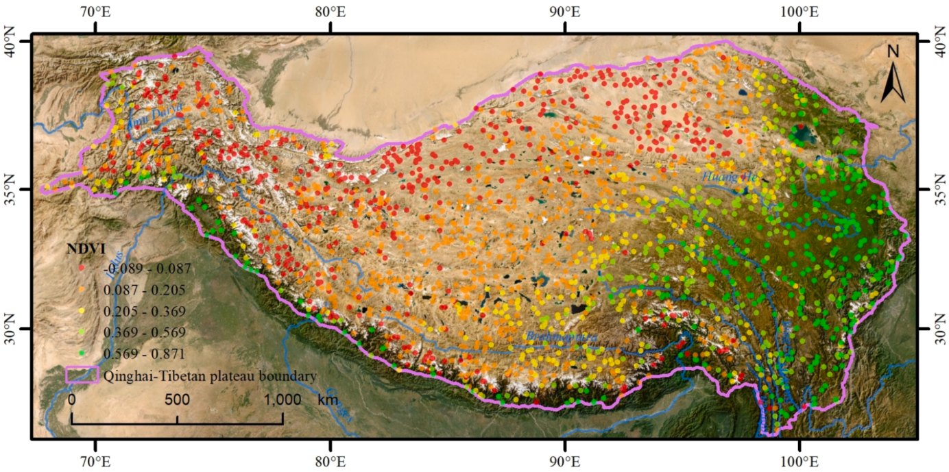
1,801 locations, not the 2,000 the article describes. The distributed file is what the pipeline reads, so every number here rests on 1,801.
328 locations have no λ at all, and only 1,283 carry a complete set of p-values. The share-significant column of Table 2 is computed over those 1,283, not over all 1,801 — getting this denominator right is what makes 94.39 %, 70.07 % and the rest come out to the printed decimal.
A quarter of the estimates fall outside [−1, 1], reaching +3,910 on the
climate-to-plant path. Table 2 and Fig. 5 describe only the estimates inside that window,
which is the filter the authors' own script applies. figs/fig07 shows how much of
each pathway that removes.
2.4 The Model Specification, and Why It Is a Reconstruction
Fig. 5 of the article draws the model: four measurement arrows into three latent variables, and three structural arrows between them. Read literally, it does not identify.
A latent variable measured by a single indicator — Plant by NDVI alone, Soil by water content alone — has its loading fixed at 1 by convention, because there is nothing to estimate it against. The published output contradicts that in two places at once: the NDVI loading varies from 0.004 to 1.000 across locations, and the water-content loading is negative at most of them, averaging −0.763. Fitting the diagram as drawn confirms it — both loadings come back as exactly 1.000 everywhere, and the structural coefficients blow up past ±900 as the optimiser works on an underdetermined problem.
The data file resolves it. It carries three variables no arrow in Fig. 5 uses — EVI, T and PH — and giving each latent a second indicator makes every loading free, negative loadings possible, and the whole model identified:
SEM_MODEL <- '
  Plant   =~ EVI + NDVI          # EVI is the reference indicator
  Climate =~ T + LST + P         # T  is the reference indicator
  Soil    =~ PH + watercontent   # PH is the reference indicator

  Soil  ~ Climate                # lambda_7
  Plant ~ Climate + Soil         # lambda_6, lambda_5
'
The reference indicators are what the published signs imply. With temperature anchoring Climate, land surface temperature loads positively (published mean +0.798) and precipitation negatively (−0.370), which is the pattern of a cold arid plateau. With pH anchoring Soil, water content loads negatively (−0.763). Fitted this way, the model returns coefficients of the right sign and the right magnitude at most locations.
The reconstruction is consistent with everything observable in the released material, and it
is still a guess about a file that was never released. If you have the authors' original
lavaan specification, replacing SEM_MODEL in the config is the whole
change required — the pipeline reads the seven pathways from PATHS and needs no
other edit.
3 Reproduction Pipeline, Results & Validation
3.1 Pipeline Execution
| Full run | Rscript run-all.R (~11 min, almost all of it Steps 30 and 50) |
|---|---|
| Verification | Rscript run-all.R test — 2 s, do this first |
| Output folders | results/ tables/ figs/ data/derived/ |
cd LPA                     # this folder
Rscript run-all.R test     # 1. check against the published values (2 s)
Rscript run-all.R          # 2. full pipeline (~11 min)

Rscript run-all.R 20 40    # re-run single steps (10 20 30 40 50 90)
Rscript run-all.R figures # only the figure scriptsProject : lpa-demo
Domain : Tibetan Plateau ecosystem (NDVI, LST, precipitation, soil water)
== Step 10 — prepare data ================================
1801 locations, 27 columns, coordinates in km
extent: 67.95 to 104.11 E, 26.21 to 39.80 N
plane : 3341 km east-west by 1503 km north-south
published lambda present at 1473 of 1801 locations (328 incomplete)
published p-values complete at 1283 locations — Table 2's denominator
== Step 20 — optimal local range =========================
L peaks at r = 705.29 km (correction 'border', rectangle window), L_max = 128.94
local range carried forward: 705.29 km (published 707.29 km, -2.00 km)
neighbourhood size: median 596, range 163-909; 0 locations below the minimum of 60
== Step 30 — local path coefficients =====================
radius 705.29 km, 1801 locations
finished in 441 s
converged at 1667 of 1801 locations (92.6 %)
== Step 40 — reproduce the published values ==============
7 of 7 rows reproduce every printed figure exactly
sign agreement 72-100 %, correlation -0.13-0.83 across the seven paths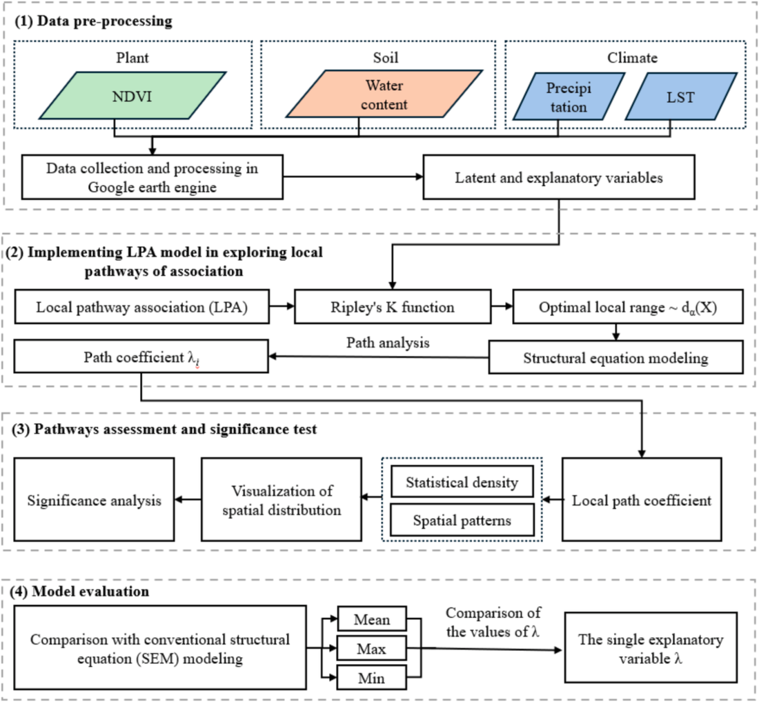
R/10, the LPA model is R/20 and
R/30, assessment and significance are R/40 with the figure scripts, and
the comparison against conventional SEM is the last column of Table 2. Click to enlarge.
Hu, Qu, Song & Wu (2025), IJAEOG 139:104531 (open access, CC BY).3.2 Reproduce the Published Values
Table 2 — reproduced exactly, once two conventions are right
Table 2 of the article validates LPA by putting the local coefficients beside the global ones. Every figure it prints follows from the distributed output file, but only under two conventions the table itself does not state, and both have to be right at once or nothing matches.
- The summaries cover only λ inside [−1, 1]. This is the filter in the authors' own plotting script. Applied to the raw columns instead, the mean for the climate-to-plant path is +3.57 rather than the published +0.335.
- The share significant is taken over the 1,283 locations with a complete set of p-values, not over all 1,801 and not over the filtered subset. Using the filtered subset instead moves four of the seven percentages off the printed value.
== test-01: published values ==================================
   [ok] lambda1 mean                       got    -0.370  want    -0.370
   [ok] lambda1 min                        got    -0.967  want    -0.967
   [ok] lambda1 max                        got     0.747  want     0.747
   [ok] lambda1 significant %              got    94.388  want    94.390
   [ok] lambda2 mean                       got     0.798  want     0.798
   [ok] lambda3 mean                       got    -0.763  want    -0.763
   [ok] lambda4 mean                       got     0.773  want     0.773
   [ok] lambda4 min                        got     0.004  want     0.004
   [ok] lambda5 significant %              got    70.070  want    70.070
   [ok] lambda6 significant %              got    63.523  want    63.520
   [ok] lambda7 significant %              got    62.354  want    62.350
   [ok] optimal local range (km)           got   705.290  want   707.290
   [ok] locations in the file              got  1801.000  want  1801.000
   [ok] locations with a complete set of p-values  got 1283.000  want 1283.000

   31 passed, 0 failed
every published figure reproduced| Path | Local λ, mean [min, max] | Significant (p < 0.05) | Global λ | Match |
|---|---|---|---|---|
| Variable relationship | ||||
| λ₁ Precipitation =~ Climate | −0.370 [−0.967, 0.747] | 94.39 % | −0.332** | exact |
| λ₂ LST =~ Climate | 0.798 [−0.605, 0.999] | 98.29 % | 0.858** | exact |
| λ₃ Water content =~ Soil | −0.763 [−0.987, 0.430] | 96.80 % | −0.895** | exact |
| λ₄ NDVI =~ Plant | 0.773 [0.004, 1.000] | 98.21 % | 0.995** | exact |
| Latent variable relationships | ||||
| λ₅ Soil ~ Plant | −0.269 [−0.998, 0.774] | 70.07 % | −0.528** | exact |
| λ₆ Climate ~ Plant | 0.335 [−0.994, 0.998] | 63.52 % | 0.267** | exact |
| λ₇ Climate ~ Soil | 0.427 [−0.969, 0.997] | 62.35 % | 0.677** | exact |
The seven pathways: local coefficient distributions, the share of locations where each is significant, and the published global coefficient beside each one. Every printed figure matches the published Table 2.
42 assertions pass — 31 against the published article, 11 on properties the method must satisfy regardless of dataset. If those hold, the pipeline is reading the case the authors published and summarising it the way they did. On a fresh unpack the tests prepare what they need and run 39 of the 42 in under a second; the remaining three compare against the local fits, so they appear once Step 30 has run.
What the global column already tells you
Read the table's last two columns together and the argument for the method appears without any map. Every global coefficient is significant at p < 0.01, yet the local range around it crosses zero on six of the seven pathways. The global −0.528 for soil on plant is the average of a surface running from −0.998 to +0.774, and the pathway is significant at only 70 % of locations. The global estimate is not wrong; it is a summary of something that has no single value.
3.3 Core Analytical Steps
Five stages: purpose → code → output → result → how to read it. Step numbers
match the script numbers (Step 1 is R/20-optimal-range.R).
Identify the optimal local range
What this step does
Ripley's K counts how many neighbours a typical location has within each distance r, and compares that count to what complete spatial randomness would give. Besag's L rescales the comparison so it can be read against zero, and the distance at which L peaks is taken as the range over which spatial interaction is strongest. That distance becomes the radius of every local model in Steps 2 and 3, which makes this the single most consequential number in the pipeline.
Code
ripley_L <- function(d, correction = K_CORRECTION, window = K_WINDOW,
                     r_max = K_R_MAX, r_step = K_R_STEP) {
  W <- if (identical(window, "hull"))
    spatstat.geom::convexhull.xy(d$px, d$py)
  else
    spatstat.geom::owin(range(d$px), range(d$py))
  pp <- spatstat.geom::ppp(d$px, d$py, window = W, checkdup = FALSE)
  K  <- spatstat.explore::Kest(pp, correction = correction,
                               r = seq(0, r_max, by = r_step))
  col <- setdiff(names(K), c("r", "theo"))[1]
  L   <- sqrt(K[[col]] / pi) - K$r          # Besag's L
  i   <- which.max(L)                       # the optimal local range
  list(r = K$r, K = K[[col]], theo = K$theo, L = L,
       r_opt = K$r[i], L_max = L[i], correction = correction)
}
Example output
== Step 20 — optimal local range =========================
   L peaks at r = 705.29 km (correction 'border', rectangle window), L_max = 128.94
   L is within 5 of its maximum from 687 to 723 km — the peak is a plateau 36 km wide
   the border correction stops being reliable beyond 751 km
   wrote results/ripley-k-curve.csv (1201 rows)
   wrote results/optimal-range.csv (4 rows)
 correction    window r_opt_km   L_max published_km difference_km selected
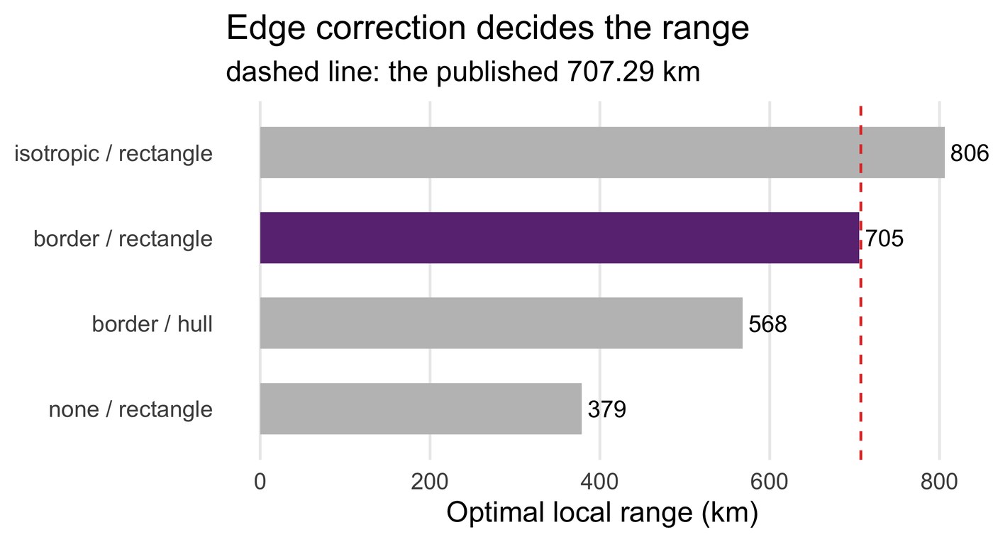
       none rectangle   378.51  62.990       707.29       -328.78    FALSE
     border rectangle   705.29 128.942       707.29         -2.00     TRUE
  isotropic rectangle   805.99  98.027       707.29         98.70    FALSE
     border      hull   568.03  48.920       707.29       -139.26    FALSE
 plateau_from_km plateau_to_km
              NA            NA
          686.95        723.18
              NA            NA
              NA            NA
   local range carried forward: 705.29 km (published 707.29 km, -2.00 km)
   neighbourhood size: median 596, range 163-909; 0 locations below the minimum of 60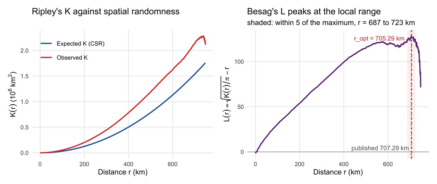
How to read this result
The reproduction lands 2 km from the published value, a difference of 0.3 %, and that residual is a projection choice the article does not state: scaling longitude by cos(latitude) gives 705.29 km, treating both axes at 111.32 km per degree gives 710.11 km, and the published number sits between them.
Agreeing to 2 km is less impressive than it sounds, and the shaded band in the figure is why. L stays within 5 units of its maximum from 687 to 723 km, so the curve has a plateau rather than a spike, and any radius in that 36 km window is an equally good reading of the same data. The honest statement is that the published range and this one fall on the same plateau — not that the third decimal was recovered.
The figure stops at 748 km although the search grid runs to 1,200. The border
correction only counts points whose whole neighbourhood of radius r lies inside the
window, and by 750 km almost none do: K falls from 2.28 million to 1.54 million in a
single step and L drops to −50. That last stretch is the estimator running out of data,
not the plateau ending, so trim_collapse() removes the collapsing tail before
plotting. The peak is unaffected — it sits 43 km before the cut — but a figure drawn
without the trim shows one cliff and nothing else.
Without a correction, pairs that fall outside the study window are simply never counted, K is biased downwards, and the peak lands at 378 km — a local model built on that radius would use a quarter of the data and answer a different question. Ripley's isotropic correction gives 806 km. The convex hull as window gives 568 km. Only the reduced-sample border correction on the bounding box reproduces the article. Report which one you used; the number means little without it.
Note also where the estimator stops: the border correction cannot estimate K beyond
750 km for this window, so the peak at 705 km sits 44 km inside the
limit of what is observable. tests/test-02 asserts that margin, because a
peak resting on the last estimable distance would be an artefact of the estimator rather
than a feature of the pattern.
Examine the local path at one location
What this step does
Around a single location, collect every observation within the radius and fit the structural
equation model to that subset alone. Nothing about the estimator changes — this is
lavaan::sem() exactly as it would be used on a whole dataset. What changes is
which rows it sees, and that is the entire methodological idea.
Code
# Every location within radius r of location i, itself included.
# This one line is what makes a path coefficient local.
neighbours_within <- function(d, i, r) {
  which(sqrt((d$px - d$px[i])^2 + (d$py - d$py[i])^2) <= r)
}

fit_local_sem <- function(dat, model = SEM_MODEL, paths = PATHS) {
  fit <- try(suppressWarnings(lavaan::sem(model, data = dat)), silent = TRUE)
  if (inherits(fit, "try-error")) return(...)            # keep NA, record why
  if (!lavaan::lavInspect(fit, "converged")) return(...)  # do not invent a number
  est <- lavaan::standardizedSolution(fit)
  # pull the seven reported pathways by their lavaan names
  mapply(function(l, o, r) est$est.std[est$lhs == l & est$op == o & est$rhs == r],
         paths$lhs, paths$op, paths$rhs)
}
Example output
lavaan 0.7-2 ended normally after 80 iterations

  Estimator                                         ML
  Number of model parameters                        17
  Number of observations                           596

Latent Variables:
                   Estimate  Std.Err  z-value  P(>|z|)   Std.lv  Std.all
  Plant =~
    EVI               1.000                               0.600    0.929
    NDVI              1.135    0.020   58.059    0.000    0.681    1.052
  Climate =~
    T                 1.000                               0.291    0.484
    LST               3.844    0.339   11.347    0.000    1.117    1.207
    P                -1.194    0.109  -10.909    0.000   -0.347   -0.409
  Soil =~
    PH                1.000                               0.682    0.857
    watercontent     -1.203    0.042  -28.778    0.000   -0.821   -0.895

Regressions:
                   Estimate  Std.Err  z-value  P(>|z|)   Std.lv  Std.all
  Soil ~
    Climate           1.438    0.114   12.618    0.000    0.612    0.612
  Plant ~
    Climate           0.707    0.078    9.070    0.000    0.343    0.343
    Soil             -0.662    0.049  -13.400    0.000   -0.753   -0.753

Warning message:
lavaan->lav_object_post_check():
   some estimated ov variances are negative
How to read this result
The Std.all column is what LPA keeps. Four of its values here — the
precipitation loading of −0.409, the LST loading of 1.207, the water-content loading of −0.895
and the NDVI loading of 1.052 — are λ₁ to λ₄ at this one location, and the three regressions
are λ₇, λ₆ and λ₅ in that order. Repeating this fit 1,801 times is the whole of Step 3.
Two standardised loadings here exceed 1, and the warning at the foot of the output explains why: the fit has assigned negative residual variance to NDVI and LST. A negative variance is impossible, so this is a Heywood case — the model is straining against a neighbourhood in which two indicators are almost perfectly collinear. lavaan reports the estimate anyway rather than refusing.
That is the mechanism behind the out-of-range values in the published output too, and it is worth naming rather than filtering silently. A λ of 1.05 is a strained fit; a λ of 3,910 is a fit that has failed while still returning a number.
134 of the 1,801 neighbourhoods do not converge, and the pipeline records NA rather than
a number for those. The published output has the same behaviour on a larger scale — 328
locations with no coefficient at all — so a gap in the map is a result, not a bug. What
matters is that the gaps are reported: results/local-fit-diagnostics.csv
carries the neighbourhood size and failure reason for every location.
Local pathway analysis across space
What this step does
Repeat Step 2 at every location. Each of the seven path coefficients stops being a scalar and becomes a surface, λij(u), which can be mapped and summarised like any other spatial variable.
Code
for (k in seq_along(idx)) {
  i   <- idx[k]
  sub <- d[neighbours_within(d, i, R_OPT), SEM_VARS, drop = FALSE]
  sub <- sub[stats::complete.cases(sub), , drop = FALSE]
  if (nrow(sub) < MIN_LOCAL_N) {                 # too few neighbours to trust
    diag_n[k] <- nrow(sub); diag_note[k] <- "too few neighbours"; next
  }
  f <- fit_local_sem(sub)
  L[k, ] <- f$lambda; P[k, ] <- f$p              # seven coefficients, seven p-values
  diag_n[k] <- f$n; diag_ok[k] <- f$converged
}
Example output
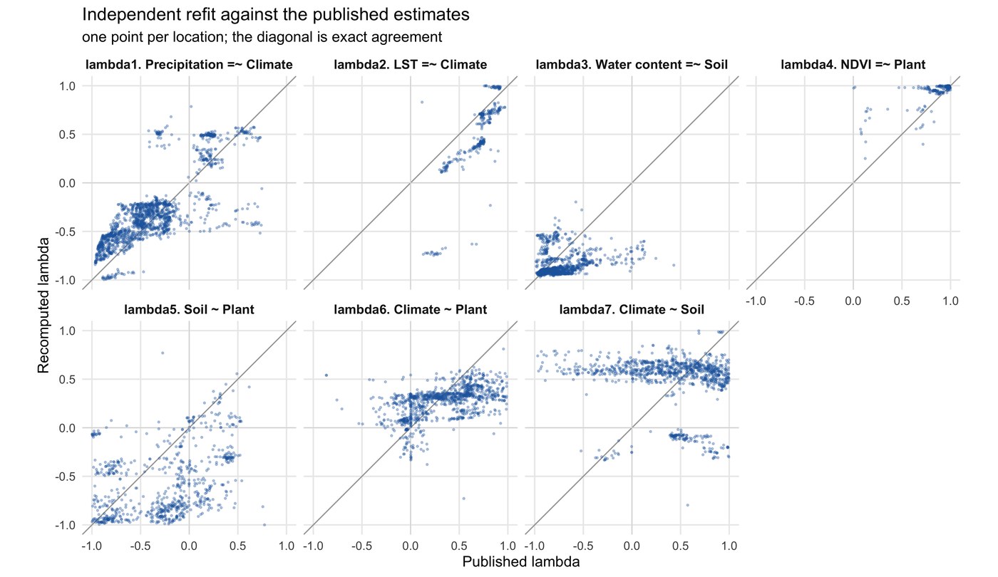
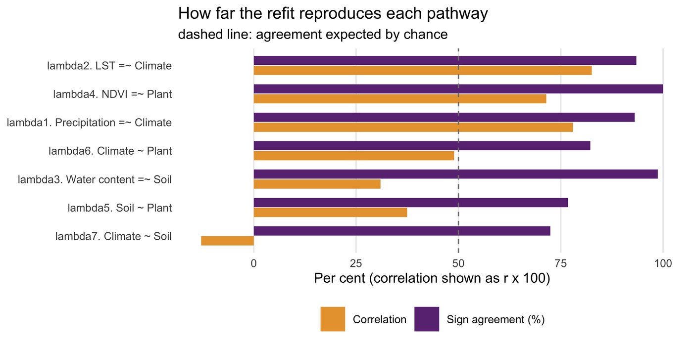
  lambda                     path        kind  n_compared  correlation  sign_agreement
 lambda1 Precipitation =~ Climate Measurement        1612        0.779            93.1
 lambda2           LST =~ Climate Measurement         306        0.826            93.5
 lambda3    Water content =~ Soil Measurement        1362        0.310            98.7
 lambda4            NDVI =~ Plant Measurement         380        0.714           100.0
 lambda5             Soil ~ Plant  Structural         731        0.374            76.7
 lambda6          Climate ~ Plant  Structural        1061        0.489            82.2
 lambda7           Climate ~ Soil  Structural        1023       -0.128            72.4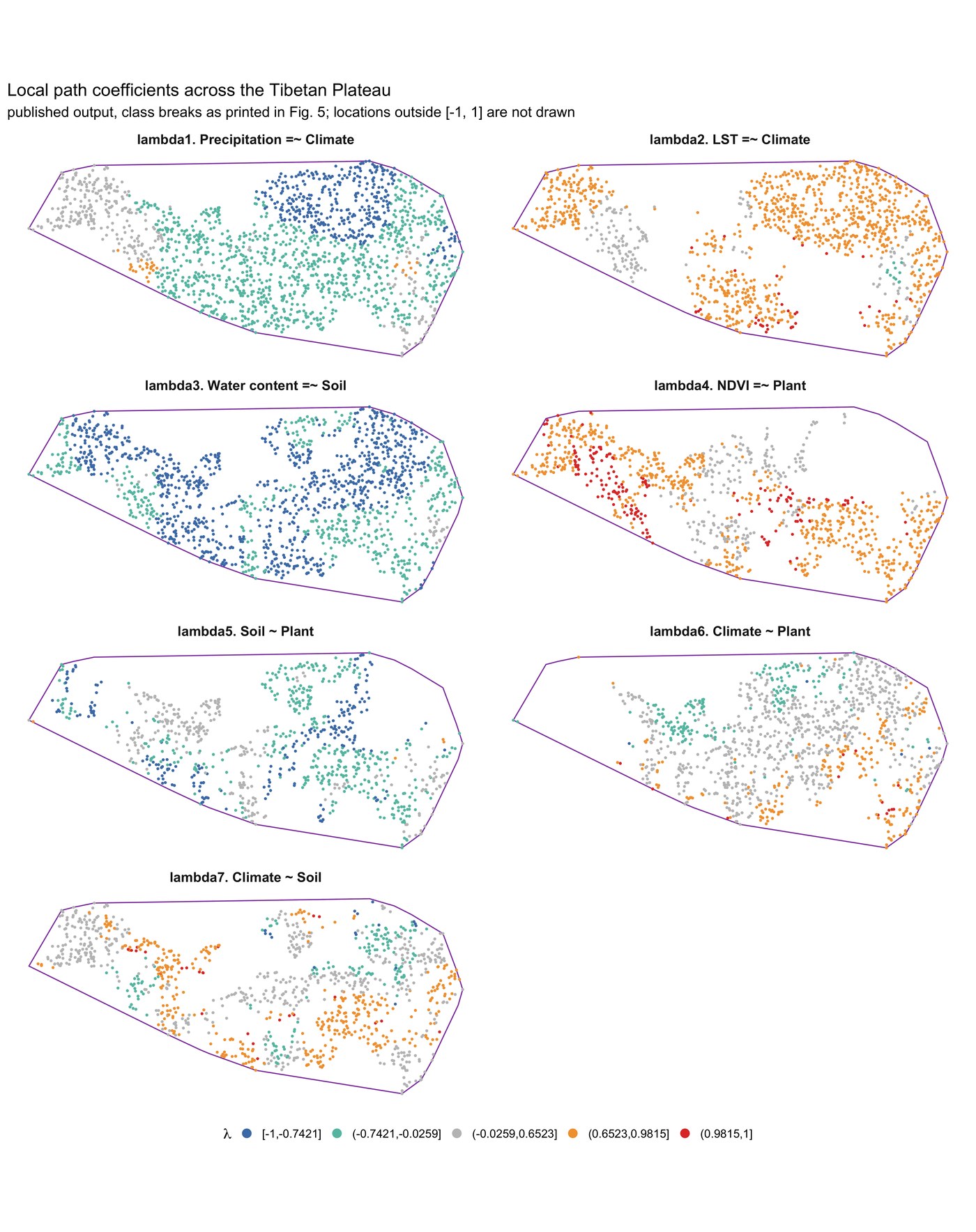
How to read this result
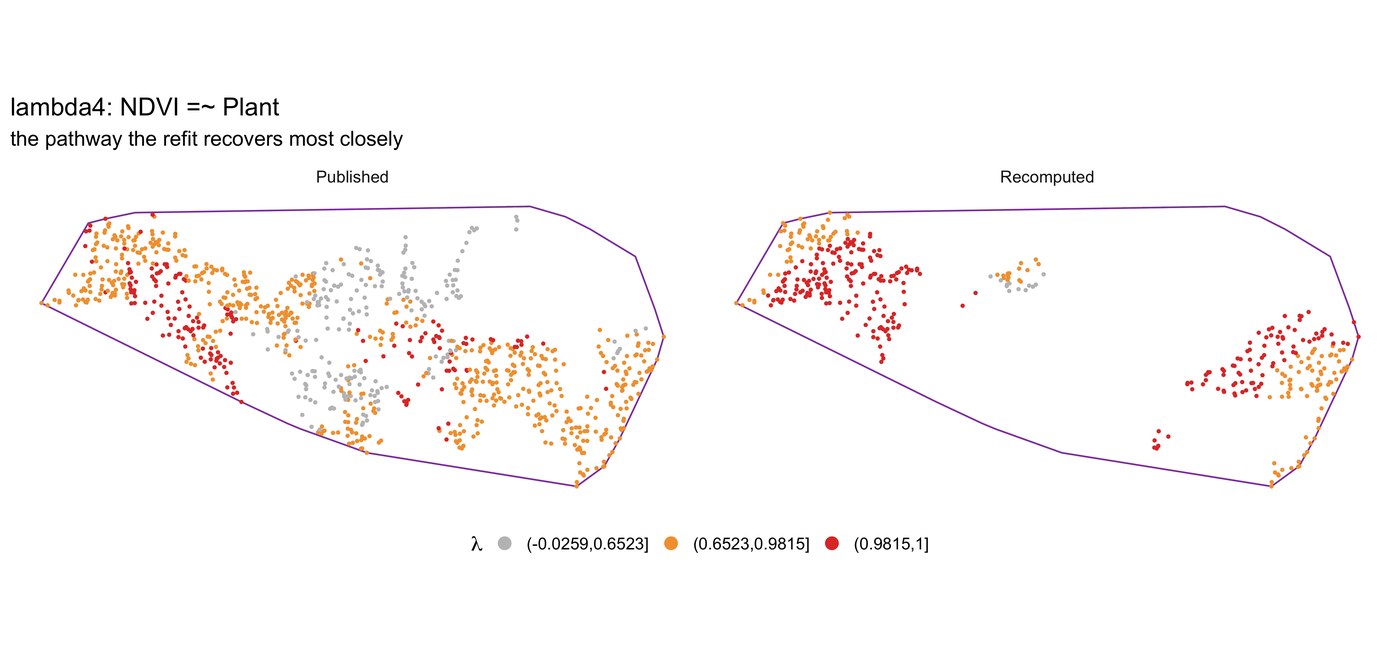
The refit reproduces the measurement half of the model well and the structural half poorly. The four measurement pathways agree in sign at 93–100 % of locations and correlate 0.31 to 0.83; the three structural pathways agree in sign at 72–82 % and one of them, climate on soil, does not correlate at all. Weighted across every comparable location, sign agreement is 87.8 %.
Loadings are pinned by the correlation between an indicator and its latent, so a measurement path is robust to how the rest of the model is written. A structural path between two latents depends on how both latents were constructed, so any difference in the specification propagates straight into it. The pattern in the table is what you would expect if the reconstruction in §2.4 has the right variables and not quite the right model — which is exactly the claim being made for it. Read the structural surfaces on this page as the published ones (they are, in fig03); read the refit as evidence that the method behaves as described, not as an independent confirmation of the estimates.
Pathway assessment and significance
What this step does
Three questions of the seven surfaces: what does the distribution of each coefficient look like, where is it significant, and how much of the study area does it actually describe.
Code
# Table 2's summary: mean [min, max] over the plotted range, and the share of
# locations whose p-value clears SIG_LEVEL — over a different denominator.
summarise_lambda <- function(lambda, p, range = LAMBDA_PLOT_RANGE,
                             alpha = SIG_LEVEL) {
  v  <- lambda[is.finite(lambda) & lambda >= range[1] & lambda <= range[2]]
  pv <- p[is.finite(p)]
  data.frame(n_in_range = length(v), mean = mean(v), min = min(v), max = max(v),
             n_p = length(pv), pct_significant = 100 * mean(pv < alpha))
}
Example output
  lambda                     path    n n_kept pct_kept        min       max
 lambda1 Precipitation =~ Climate 1732   1732   100.00 -9.665e-01    0.7466
 lambda2           LST =~ Climate 1732   1212    69.98 -6.052e-01   21.8025
 lambda3    Water content =~ Soil 1475   1472    99.80 -1.364e+00    0.4304
 lambda4            NDVI =~ Plant 1801   1015    56.36  3.525e-03   10.3234
 lambda5             Soil ~ Plant 1475    906    61.42 -5.439e+02 1564.6905
 lambda6          Climate ~ Plant 1732   1164    67.21 -6.477e+02 3910.1002
 lambda7           Climate ~ Soil 1473   1145    77.73 -1.353e+02   38.0763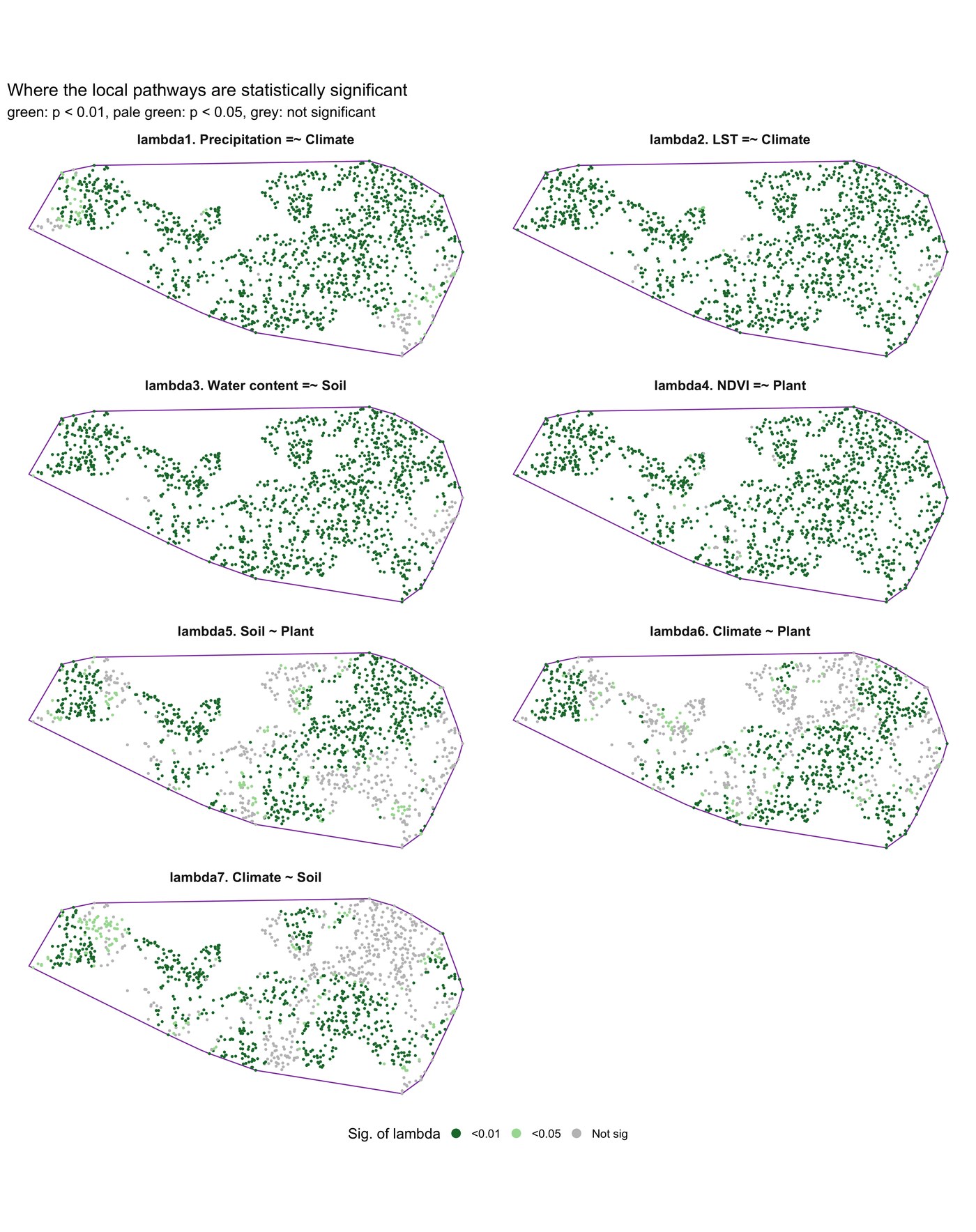
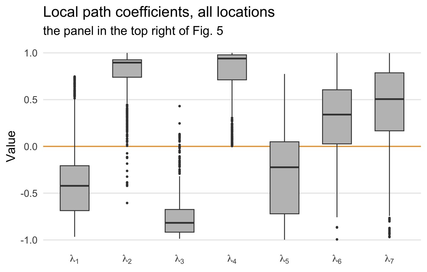
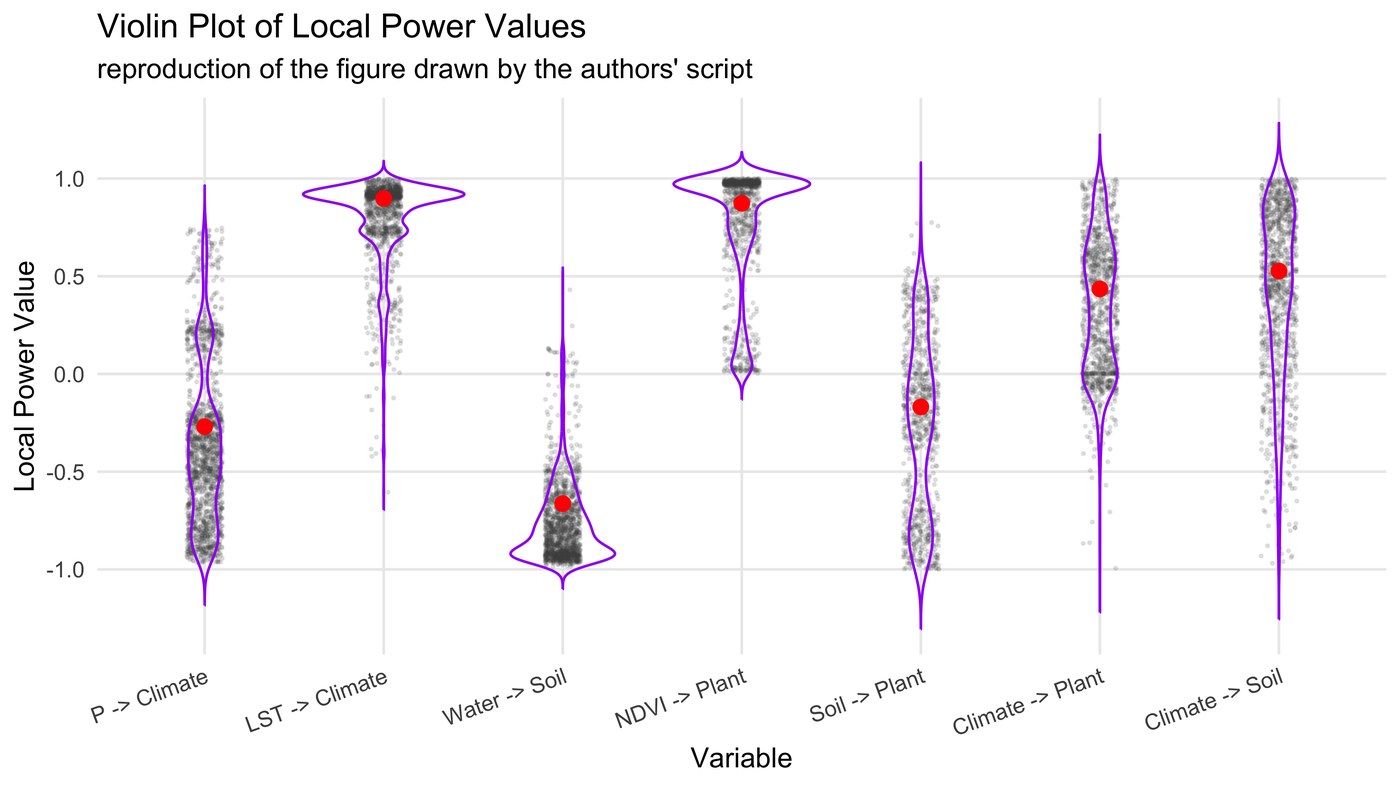
data/original-violin-plot.R as they wrote it: jittered points, purple violins,
red mean markers nudged upwards.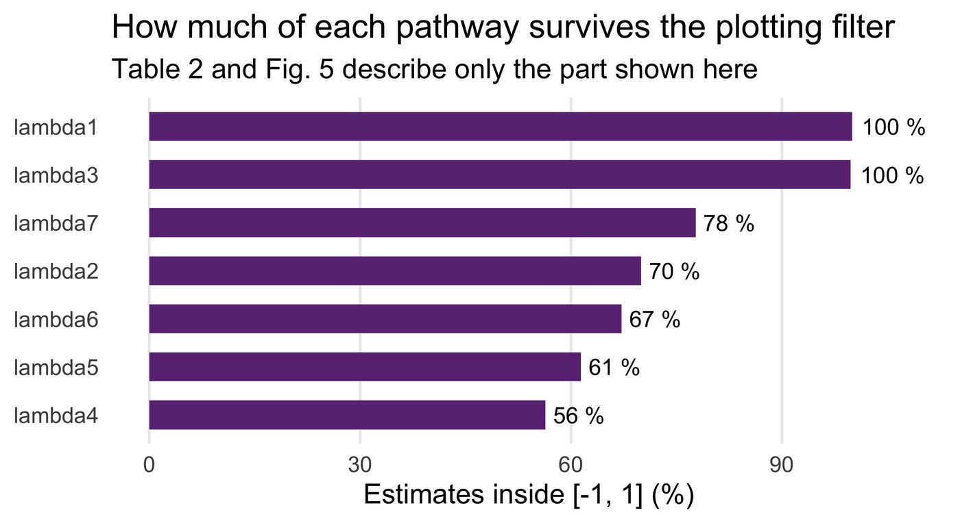
How to read this result
Two of these panels carry a warning rather than a finding. The maps in fig03 and fig04 look
complete, but λ₄ is drawn at 56 % of locations and λ₅ at 50 % — the rest are either
missing or outside the plotted range. A reader of the published figure has no way to tell the
difference between a location that was estimated as unremarkable and one that was dropped, so
results/map-coverage.csv reports the coverage of every panel explicitly.
Model evaluation, and the cost of the radius
What this step does
The article evaluates LPA by comparing local coefficients against global ones. This pipeline adds the check the article's own limitations section asks for: how much of the answer is decided by the radius chosen in Step 1.
Code
RADIUS_SENSITIVITY <- c(400, 500, 600, 705.29, 800, 900)

# Fitting every location at six radii would take the best part of an hour,
# so the check runs on a fixed random subsample.
for (r in RADIUS_SENSITIVITY) {
  for (k in seq_along(idx)) {
    sub <- d[neighbours_within(d, idx[k], r), SEM_VARS, drop = FALSE]
    f <- fit_local_sem(sub[stats::complete.cases(sub), , drop = FALSE])
    L[k, ] <- f$lambda
  }
}
Example output
== Step 50 — radius sensitivity ==========================
   150 locations at 6 radii: 400, 500, 600, 705.29, 800, 900 km
   r = 400.00 km: median 248 neighbours, 88 % converged, mean |lambda| sd 0.286
   r = 500.00 km: median 362 neighbours, 88 % converged, mean |lambda| sd 0.334
   r = 600.00 km: median 480 neighbours, 92 % converged, mean |lambda| sd 0.270
   r = 705.29 km: median 604 neighbours, 93 % converged, mean |lambda| sd 0.254
   r = 800.00 km: median 723 neighbours, 92 % converged, mean |lambda| sd 0.222
   r = 900.00 km: median 870 neighbours, 94 % converged, mean |lambda| sd 0.222
   wrote results/radius-sensitivity.csv (42 rows)
   Precipitation =~ Climate mean lambda -0.381 to -0.298 across radii, sign stable
   LST =~ Climate           mean lambda  0.184 to  0.752 across radii, sign stable
   Water content =~ Soil    mean lambda -0.888 to -0.825 across radii, sign stable
   NDVI =~ Plant            mean lambda  0.869 to  0.988 across radii, sign stable
   Soil ~ Plant             mean lambda -0.649 to -0.348 across radii, sign stable
   Climate ~ Plant          mean lambda  0.258 to  0.307 across radii, sign stable
   Climate ~ Soil           mean lambda  0.480 to  0.636 across radii, sign stable
The same 42 rows, pivoted to one row per radius — this is what
tables/table-radius-sensitivity.tex typesets:
| Radius (km) | Median neighbours | λ₁ | λ₂ | λ₃ | λ₄ | λ₅ | λ₆ | λ₇ |
|---|---|---|---|---|---|---|---|---|
| 400 | 248 | −0.381 | 0.752 | −0.829 | 0.869 | −0.348 | 0.301 | 0.636 |
| 500 | 362 | −0.314 | 0.498 | −0.825 | 0.910 | −0.424 | 0.307 | 0.552 |
| 600 | 480 | −0.349 | 0.508 | −0.856 | 0.951 | −0.517 | 0.273 | 0.575 |
| 705.29 | 604 | −0.350 | 0.419 | −0.875 | 0.933 | −0.578 | 0.272 | 0.538 |
| 800 | 723 | −0.310 | 0.350 | −0.875 | 0.983 | −0.625 | 0.269 | 0.487 |
| 900 | 870 | −0.298 | 0.184 | −0.888 | 0.988 | −0.649 | 0.258 | 0.480 |
Radius sensitivity: the seven mean path coefficients recomputed at six local ranges. Signs are stable throughout; two of the seven magnitudes are not.
How to read this result
No pathway changes sign anywhere between 400 and 900 km, which is the reassuring half of the result: the direction of every arrow is a property of the plateau rather than of the radius. The magnitudes are another matter. Three pathways barely move — precipitation on climate, water content on soil, climate on plant all shift by less than 0.09 — while the LST loading falls from 0.752 to 0.184 as the window widens, and soil on plant nearly doubles in strength. Both drift monotonically, which is the signature of a coefficient being averaged over progressively more heterogeneous territory rather than of noise.
Agreement with the published surfaces is also highest near the chosen radius: correlations for the LST and NDVI loadings peak at 600–705 km (0.90 and 0.91 at 600 km) and fall away at 800 and 900 km. That is weak independent support for 707.29 km being the radius behind the published numbers, arrived at without using it.
The article's limitations section notes that choosing a different local range may change the results, and leaves it there. Running the model at five more radii costs four minutes on a subsample and converts that caveat into a measurement: which of your conclusions survive the choice, and which are artefacts of it. On this case the signs survive and two of the seven magnitudes do not.
3.4 Reading the Results Together
| The pathways are local | every global coefficient is significant at p < 0.01, yet six of the seven local ranges cross zero — the strongest, soil on plant, runs from −0.998 to +0.774 around a global −0.528. |
|---|---|
| Measurement is stable, structure is not | the four indicator loadings are significant at 94.4–98.3 % of locations; the three latent-to-latent pathways at 62.4–70.1 %. Where climate acts on soil, it does so somewhere rather than everywhere. |
| And the maps are partial | between 50 % and 96 % of locations are drawn per panel once missing and out-of-range estimates are removed. Coverage belongs in the caption. |
The three findings above point the same way. LPA earns its keep not by producing a better number than a global SEM but by showing that the number was never single — and the same evidence that makes that case also limits how far any one local coefficient should be pushed. A coefficient estimated from 596 overlapping neighbours, significant at 62 % of locations, drawn on 64 % of the study area and moving by 0.16 when the radius changes is good evidence of spatial heterogeneity in the climate-to-soil pathway. It is weak evidence about any particular valley.
Claim: the association between these variables varies across the plateau by more than a global model can express, with a consistent geography — the vegetation loading strongest in the west and north, the climate–soil pathway concentrated in the centre.
Do not claim: that a coefficient at one location is an estimate for that location alone. Neighbouring fits share most of their data by construction, so the surfaces are smooth whether or not the underlying process is.
Report alongside: the radius and the edge correction that produced it, the share of locations that converged, the share drawn on each map, and the sensitivity table. Four numbers, and they turn a set of attractive maps into a result someone else can check.
4 Adaptation, Writing & Reproducibility
4.1 Port to Your Domain
LPA needs point locations, a set of observed variables and a causal diagram worth testing. It does not care whether the variables are ecological — the same structure applies to house prices and amenities, or to exposure, deprivation and health.
What to edit
| Setting | What to put there |
|---|---|
INPUT_FILE, COORD_X, COORD_Y |
your point table and its coordinate columns. Standardise the variables first; the pipeline does not do it for you. |
SEM_MODEL, SEM_VARS |
the causal diagram, in lavaan syntax. Give every latent at least two
indicators — the identification problem in §2.4 is not specific to this case. |
PATHS |
the pathways you want reported, named as lavaan names them. This drives
the tables, the maps and the tests together. |
PROJECTION |
"equirect" for a study area of a few thousand kilometres;
"degrees" if you have already projected the coordinates properly. |
K_CORRECTION, K_WINDOW |
leave at "border" and "rectangle" unless you have a reason,
and report what you used. §3.3 Step 1 shows the range these choices span. |
MIN_LOCAL_N |
the smallest neighbourhood you will accept a fit from. A structural equation model with 17 free parameters needs considerably more than 17 observations. |
RADIUS_SENSITIVITY |
a spread either side of your estimated range. Run it before you write the discussion, not after a reviewer asks. |
The configuration entries to change when porting the model to another study area. Everything else in the pipeline follows from these.
The radius swallows the study area. If the estimated range covers most of your data, every local model is nearly the global model and the surfaces will be flat. Check the median neighbourhood count that Step 20 prints before going further.
The model does not converge locally. A specification that fits the full dataset can fail on a subset with less variation. The pipeline records NA and moves on; if the failure rate is high, the specification is too ambitious for the local sample size, not the other way around.
Coefficients escape [−1, 1]. A standardised loading above one is possible with correlated factors, but a value of 3,910 is a fit that has come apart. Filtering them out for the figures is reasonable; doing so without saying how many were removed is not.
4.2 Write the Paper
Manuscript skeleton
| Section | What goes in it | From |
|---|---|---|
| Method — local range | Ripley's K, Besag's L, the correction you used and the range it gave | results/optimal-range.csv, figs/fig01 |
| Method — local model | the SEM specification and the neighbourhood rule | config/project-config.R |
| Results — the surfaces | one map per pathway, significance beside it | figs/fig03, figs/fig04 |
| Results — the summary | local mean [min, max] against the global coefficient | tables/table-lpa-validation.tex |
| Results — distribution | the boxplot, and what the plotting filter removed | figs/fig05, figs/fig07 |
| Discussion — robustness | the radius sensitivity table | tables/table-radius-sensitivity.tex |
| Limitations | convergence rate, map coverage, overlapping neighbourhoods | results/local-fit-diagnostics.csv, results/map-coverage.csv |
A manuscript skeleton for reporting an LPA analysis, with the output file behind each section.
Manuscript outline
1  Introduction       — associations between variables are assumed constant over
                         space; path analysis is global; the contribution (3 aims)
2  LPA model          — 2.1 The optimal local range (Ripley's K, Besag's L)
                         2.2 The local structural equation model
                         2.3 Estimation at every location; the surfaces
                         2.4 Assessment: significance, convergence, coverage
3  Case & data        — study area, the observed variables, the causal diagram
4  Results            — 4.1 the local range and what fixes it
                         4.2 the seven pathway surfaces and their significance
                         4.3 local against global coefficients
                         4.4 sensitivity to the radius
5  Discussion         — what varies in space and what does not; the identification
                         limits of the reconstructed specification
6  Conclusions        — the local pathways, and the radius they depend on
Questions a reviewer will ask
Why that radius? → results/optimal-range.csv shows the estimate and the three
alternatives. Would a different radius change the conclusion? →
tables/table-radius-sensitivity.tex; on this case the signs hold and two magnitudes
move. How many local models failed? → 134 of 1,801 here, in
results/local-fit-diagnostics.csv. Is the map showing every location? →
results/map-coverage.csv, and no. Is this just a global model in disguise? →
tests/test-02 checks that 59 % of locations sit more than 0.1 away from the
global estimate.
4.3 Final Reproducibility Package
| Code | numbered scripts in R/, one
command in run-all.R, every choice in config/project-config.R |
|---|---|
| Data | data/lpa-tibetan-plateau.csv
— the 1,801 published locations, carrying both the observed variables and the authors' own
output; data/LSEM_out.xlsx as distributed;
data/original-violin-plot.R unedited |
| Results | 10 CSV files in results/,
4 LaTeX tables in tables/, 10 figures in figs/ as both PDF and
PNG |
| Verification | 42 assertions —
Rscript run-all.R test — of which 31 are against the printed article; the tests
prepare their own inputs, so they run on a fresh unpack |
| Environment | env/session-info.txt,
written by every run |
References & credits
Demo outputs were generated by the scripts in this folder with R 4.6.0,
lavaan 0.7.2 and spatstat.explore 3.8.1. Reference figures are reproduced
from the article, which is open access under CC BY, for comparison. The data file and the
violin-plot script were provided by the authors.
- Hu J, Qu R, Song Y, Wu P (2025). Local pathways of association.
International Journal of Applied Earth Observation and Geoinformation 139:104531.
doi:10.1016/j.jag.2025.104531
· PDF
(source of the model, the case study, the Fig. 1, Fig. 4 and Fig. 5 reference images, and of
every value locked in
tests/test-01) - Rosseel Y (2012). lavaan: an R package for structural equation modeling. Journal of Statistical Software 48(2):1–36. doi:10.18637/jss.v048.i02 · CRAN (the estimator behind every local fit)
- Baddeley A, Rubak E, Turner R (2015). Spatial Point Patterns: Methodology and Applications with R. Chapman and Hall/CRC. spatstat (Ripley's K, and the edge corrections that decide the local range)
- Ripley BD (1977). Modelling spatial patterns. Journal of the Royal Statistical Society B 39(2):172–192. doi:10.1111/j.2517-6161.1977.tb01615.x (the K function)
- Besag J (1977). Contribution to the discussion of Dr Ripley's paper. Journal of the Royal Statistical Society B 39(2):193–195. (the L transform whose peak defines the local range)
- Anselin L (1995). Local indicators of spatial association — LISA. Geographical Analysis 27(2):93–115. doi:10.1111/j.1538-4632.1995.tb00338.x (the local-statistics tradition LPA extends to path analysis)