Reproducing the Generalized Covariate Field

1 Method Overview & Reproduction Scope

1.1 Core Idea

Most attempts to improve spatial prediction add model: a deeper forest, a cleverer kernel, another layer. GCF starts from the opposite observation — the covariates themselves carry spatial information that point values throw away. A location is not just its covariate vector: it sits inside a neighbourhood of covariate values, with local dependence, heterogeneity, multiscale variation and outlyingness of its own. The generalized covariate field (GCF) turns that surrounding structure into explanatory variables.

GCF is a feature transform, not a learner — there is no fitting inside it. Each covariate is expanded into two families of features at every location, sampled and unsampled: spatial pattern features ψ (eleven local operators over a series of buffer radii) and neighbourhood distribution features Z_x (quantiles of the covariate over multiscale neighbourhoods). The sweeps are collinear by construction, so a functional reduction compresses them into interpretable candidates, and a stability selection keeps the few that matter. Any learner then fits on raw covariates + selected features exactly as it would have fit on raw covariates alone.

• Research problem: prediction accuracy is constrained by spatial heterogeneity and sparse, uneven sampling; existing methods respond by increasing algorithmic complexity while underusing the spatial information embedded in the covariates themselves.
• One-line contribution: expand the covariate space — pattern operators + neighbourhood quantiles + leakage-free reduction + spatial-block stability selection — so that a fixed learner sees the spatial structure it could not extract from point values.
• Why it matters here: in the simulation, GCF lifts the spatial-block CV R² of every one of seven learners — RF from 0.419 to 0.657 (+56.5 %) — and the reproduction of the paper's Table 2 below is byte-identical. In the case study it lifts RF spatial R² from 0.296 to 0.346 (+16.7 %) with a 3.0 % RMSE reduction.

1.2 Method Logic

GCF runs in four steps, followed by the paper's validation design. The notation follows the paper's Section 2; every step below is exercised by the pipeline in §3.

Step 1 — spatial pattern features ψ

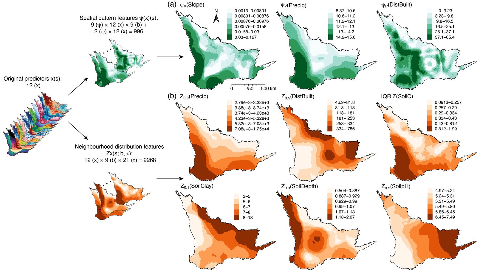
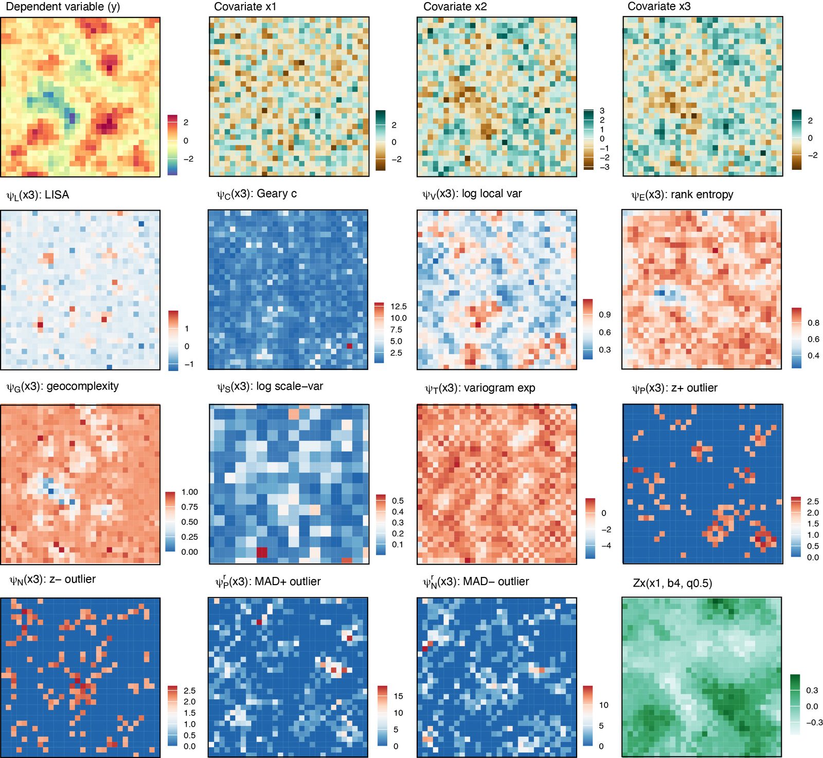
For each covariate and each buffer radius b, eleven local operators describe the covariate's spatial behaviour around location v: LISA on the local z-score (spatial dependence), local Geary's c (local contrast), log local variance (heterogeneity), rank-binned quantile entropy (local diversity), geocomplexity (single scale), log scale-variance across the scale series (single scale), the local variogram exponent (roughness of local spatial structure), and positive/negative z-score and MAD outlier strengths (local outlyingness). The simulation uses buffers {2, 4, 6} on the unit grid → 87 ψ columns from 3 covariates; the case study uses {20, …, 100} km → 12 × 83 = 996.

Step 2 — neighbourhood distribution features Z_x

For each location v, covariate x and buffer b, summarise the covariate's distribution over the support points inside the buffer by quantile levels τ:

Sim: 3 covariates × 3 buffers × 11 quantile levels = 99 columns. Case: 12 × 9 × 21 = 2,268. Together with ψ this is what "the field" in the method's name means: every covariate becomes a field of spatial descriptors around every location, computable at unsampled locations too.

Step 3a — functional reduction (leakage-free)

The quantile/buffer sweeps are strongly collinear, so they are reduced to interpretable functionals — a per-row transform computed once, with no response involved. Two scale bands are fixed a priori: fine ({20, 30} km in the case, {2} in the sim) and broad ({90, 100} km / {6}). For each covariate × band, the band-averaged quantile curve yields five D (context) functionals:

and each buffered ψ operator is band-averaged into P (pattern) candidates (the two single-scale operators pass through). Together with the raw covariates X, the reduced candidate field is 93 columns in the sim (X 3, P 60, D 30) and 372 in the case (X 12, P 240, D 120) — the paper's Table 4, which step 4 regenerates byte-for-byte.

Step 3b — selection: rf_imp kernel + spatial-block stability + group voting

Selection runs on training rows only (inside each CV fold, so it is leakage-safe). Three moves:

1. Per-subsample selector. On a subsample, fit a random forest (ranger, 200 trees) and keep the top K = 20 derived features by impurity importance: s_b,j = 1{rank(−imp_j) ≤ 20}. The raw covariates are always kept.
2. Spatial-block stability. The training rows fall in spatial blocks; for b = 1…B (B = 80) draw ⌊0.7 M⌋ of the M blocks, run the selector, and record the selection frequency freq_j = (1/B) Σ_b s_b,j.
3. Medium group voting. Group the derived features by (covariate × category). A group qualifies if any member is kept in at least π = 0.6 of the resamples — fire_g = (1/B) Σ_b 1{Σ_j∈Gg s_b,j > 0} ≥ π — and contributes its highest-frequency member. Voting de-dilutes collinear blocks: sibling features split freq so none clears π alone, while the block as a whole fires reliably.

The output S = covariates ∪ group representatives is typically ~20–25 features in the case study and 8 in the simulation.

The validation design — dual five-fold cross-validation

Two partitions of the same samples: ordinary random five-fold (interpolation), and spatial-block five-fold (transfer): square blocks of side L = 2 × the residual variogram range (132 km in the case; 6 in the sim) are assigned whole to folds by shuffled round-robin (seed 36). Metrics are per-fold mean ± sd:

Seven learners are compared, each with the paper's fixed settings — RF (randomForest, 500 trees), Cubist, GLMNET (ridge), LM, XGBoost, SVM (radial), KNN — first on the raw covariates, then on the per-fold re-selected GCF sets. Because both arms share folds and learners, any difference is attributable to the representation, not to the algorithm.

1.3 The Two Experiments — Purpose, Results, Interpretation

The paper tests GCF twice, and the two experiments answer different questions. The simulation is a controlled test of the mechanism: the truth is known, so a gain can be traced to the features that produce it. The biodiversity case is a test of usefulness: real covariates, uneven sampling, and a response nobody designed. Both are summarised here with the paper's own figures; §3 then regenerates every table quoted.

Experiment 1 — simulation on a 30 × 30 grid

Published reference · GCF Fig. 1 The simulation in one figure (Song 2026, Figure 1). Top row: the response has smooth spatial structure, while the three covariates look close to noise. Rows 2–4: the eleven spatial pattern operators applied to x₃ — each picks out a different aspect of local structure, from dependence (ψ_L, ψ_C) to outlyingness (ψ_P, ψ_N and their robust forms). Bottom right: the neighbourhood median of x₁ at buffer 4, Z_x(x₁; b = 4, τ = 0.5). Compare it with the response in the top-left panel: the pattern that a single cell of x₁ cannot show is recovered from its surroundings. Steps 1–3 run this experiment in full.

Experiment 2 — plant species richness in southwest Australia

The figure at the top of this page (the paper's Figure 5) shows where this experiment ends up: nine derived features, all at the broad 90–100 km band, join the twelve covariates in the final model. The paper's Figures 6–9 appear in steps 4–6, next to the numbers they explain.

1.4 Reproduction Scope

Everything tagged Demo run regenerates from this folder with Rscript run-all.R on R 4.6.0 with gcf 0.1.0, and every table it writes is byte-identical to the published CSV.

How to use this page

• To reproduce the demo: run Rscript run-all.R. Every table and demo figure below regenerates in about 140 seconds.
• To use GCF on your own data: §2.3 gives the data contract — one table with projected coordinates, a response at the sampled rows and covariates everywhere — and §4.1 the porting steps.

2 Setup, Structure & Data Contract

2.1 Environment & Dependencies

The method is one package written for the paper and validated bit-identical against its analysis engine; the learners are the seven the paper compares.

# The method, and both input data sets (from CRAN)
install.packages("gcf")
# The seven learners of the per-model comparison
install.packages(c("ranger", "randomForest", "glmnet", "Cubist",
                   "xgboost", "e1071", "kknn"))

2.2 Project Structure & Configuration

One entry script runs the six numbered steps and the table builder. Each step writes to results/, tables/, figs/ or data/derived/ and reads what the previous step wrote, so any step can be re-run in isolation after a configuration change.

GCF/
├── gcf.html                       # this guide
├── run-all.R                      # entry point: full run or single steps
├── config/project-config.R        # the ONLY file to edit for a new domain
├── R/
│   ├── 00-config.R, 01-helpers.R  # paths, IO, folds, the 7 learners, base-R maps
│   ├── 10-sim-field.R             # sim: gcf_field -> 93 candidates + full-data selection
│   ├── 20-sim-cv.R                # sim: dual five-fold design + 10 per-fold selections
│   ├── 30-sim-permodel.R          # sim: 7 learners x base/GCF  ->  Table 2
│   ├── 40-case-field.R            # case: gcf_field on the 958 observed cells -> Table 4
│   ├── 50-case-tables.R           # case: Tables 5-7 from case_final.rds
│   ├── 60-case-prediction.R       # case: both prediction surfaces, mapped
│   └── 90-tables.R                # LaTeX tables + session info
├── data/                          # sim-grid.csv + bio-grid.csv (written by steps 1 and 4),
│                                  #   case_final.rds, paper-tables/, provenance.md
├── tests/                         # bundled test scripts
├── env/                           # requirements.md, runtimes.csv, session-info.txt
└── results/  tables/  figs/       # generated output, never hand-edited

Main configuration file

config/project-config.R is the single file a reader edits. Every value in it is the paper's setting; nothing else in the pipeline hard-codes a column name, a buffer or a seed.

# -- Simulation --------------------------------------------------------------
SIM_VARS    <- c("x1", "x2", "x3");  SIM_Y <- "y1";  SIM_COORDS <- c("x", "y")
SIM_BUFFERS <- c(2, 4, 6)          # buffer radii, grid units
SIM_PROBS   <- seq(0, 1, 0.1)      # 11 quantile levels for the Zx sweep
SIM_D_NORM  <- 4                   # normalisation distance (middle buffer)
SIM_FINE    <- 2;  SIM_BROAD <- 6  # reduction bands {2} / {6}
SIM_L       <- 6                   # spatial-block side

# -- Case study ---------------------------------------------------------------
CASE_BUFFERS <- seq(20, 100, 10)   # 9 buffer radii, km
CASE_PROBS   <- seq(0, 1, 0.05)    # 21 quantile levels
CASE_D_NORM  <- 100                # km
CASE_FINE    <- c(20, 30);  CASE_BROAD <- c(90, 100)
CASE_L       <- 132                # block side, km (2 x variogram range 66)

# -- Selection (rf_imp + spatial-block stability + group voting) --------------
SEL_B    <- 80L;   SEL_FRAC  <- 0.7;  SEL_PI   <- 0.6
SEL_KTOP <- 20L;   SEL_TREES <- 200L; SEL_SEED <- 1L

# -- Cross-validation ---------------------------------------------------------
K_FOLDS <- 5L;  SEED_SHUF <- 36L;  SEED_RANDOM <- 1L

# -- Learners -----------------------------------------------------------------
LEARNERS <- c("RF", "Cubist", "GLMNET", "LM", "XGBoost", "SVM", "KNN")
RF_TREES <- 500L                   # trees of the RF learner (not the selector)

# -- Compute ------------------------------------------------------------------
CORES <- 5L   # wall clock only: every selection re-seeds its own RNG

2.3 Data Contract

GCF needs one plain table: projected coordinates, a response at the sampled rows, and covariates at every row where you want features. Unlike a purely tabular method, the coordinates are load-bearing — buffers, blocks and folds are all defined on them.

The shipped result object

3 Reproduction Pipeline, Results & Validation

3.1 Pipeline Execution

cd GCF                     # this folder
Rscript run-all.R          # full pipeline, ~140 s

Rscript run-all.R 30 50    # run single steps (10 20 30 40 50 60 90)

Project : gcf-reproduce
Domain  : sim: 30 x 30 synthetic grid | case: SWAFR plant species richness
== Step 10  Simulation: GCF candidate field ==============
   sim_grid: 900 cells, response y1, covariates x1, x2, x3
   gcf_field (psi + Zx + reduction) took 5.3 s
   candidates: 93  [X (raw) 3 | P (pattern) 60 | D (context) 30]
   gcf_select on all 900 cells (B = 80) took 12.3 s
   selected 8 variables: x1, x2, x3, x1_D_fine_med, x2_D_fine_med,
                         x2_P_gc, x3_D_fine_med, x3_P_gc
== Step 20  Simulation: CV folds + per-fold selection ====
   random folds: 180/180/180/180/180
   spatial folds (25 blocks): 180/180/180/180/180
   selected set sizes — spatial: 8/8/8/8/8 | random: 8/8/8/8/8
== Step 30  Simulation: per-model dual five-fold CV ======
   RF 5.8 s · Cubist 1.4 s · GLMNET 0.2 s · LM 0.0 s
   XGBoost 0.9 s · SVM 0.2 s · KNN 0.1 s
   best learner by spatial GCF RMSE: LM
   Table 2 vs paper: IDENTICAL byte-for-byte (max |diff| = 0)
== Step 40  Case study: GCF feature generation ===========
   bio_grid: 6229 cells, 958 observed (richness > 0)
   gcf_field on 958 cells (9 buffers, 21 quantiles) took 59.4 s
   candidates: 372  [X (raw) 12 | P (pattern) 240 | D (context) 120]
   Table 4 vs paper: IDENTICAL byte-for-byte
      selection: 21 variables

== Step 50  Case study: rebuild Tables 5-7 ===============
   table05-case-permodel vs paper: IDENTICAL byte-for-byte
   table06-case-featuresets vs paper: IDENTICAL byte-for-byte
   table07-case-shapley vs paper: IDENTICAL byte-for-byte
== Step 60  Case study: prediction surfaces ==============
   cross-section: 93 cells along lat -33.01 (ykm = -3654)
Finished in 132.3 s

3.2 Core Analytical Steps

Six steps: purpose → code → output → result → how to read it. Steps 1–3 are the simulation; steps 4–6 are the case study. Each maps one-to-one onto a numbered script.

Step 1 · R/10-sim-field.R

Simulation — build the GCF candidate field

What this step does

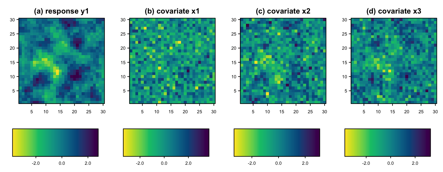
Loads the packaged 30 × 30 simulation grid (response y1 with smooth spatial structure; three covariates that are nearly unstructured at point level), writes a verbatim CSV copy, and runs the whole feature transform in one call: gcf_field() computes the eleven ψ operators over buffers {2, 4, 6}, the Z_x quantiles at 11 levels, and the functional reduction with bands {2}/{6} — 93 candidates from 3 covariates. 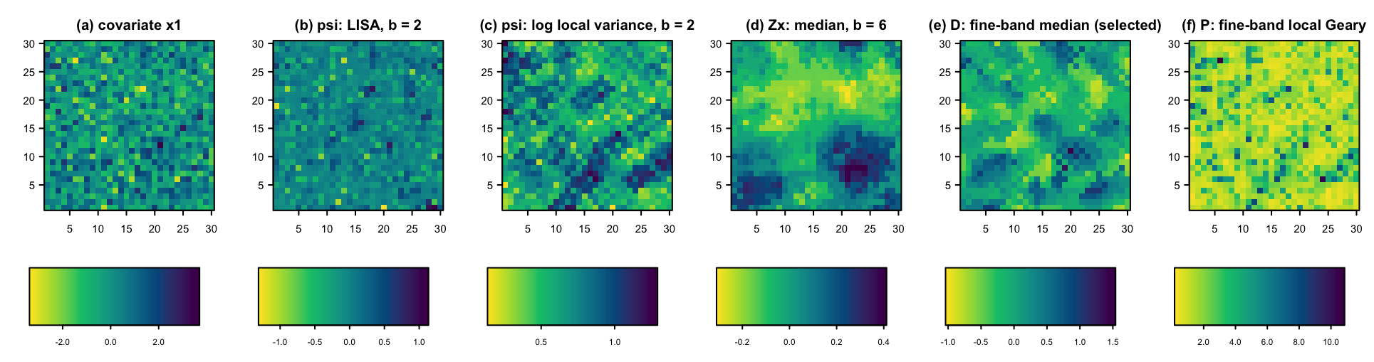It then runs one full-data B = 80 selection as a first look at what GCF keeps. The demo figures below are this pipeline's own redrawing of the paper's Figure 1 (§1.3): the same response and covariates, with x₁ traced through the transform instead of x₃.

Code

R — from R/10-sim-field.R

field <- gcf::gcf_field(sim, coords = c("x", "y"), vars = c("x1", "x2", "x3"),
                        buffers = c(2, 4, 6), probs = seq(0, 1, 0.1),
                        d_norm = 4, include_vario_exp = TRUE,
                        vario_buffers = c(2, 4, 6),
                        fine_band = 2, broad_band = 6)
# 900 x 93 candidates: field$candidates, field$meta, field$psi, field$zx

bid <- gcf::gcf_blocks(sim[, c("x", "y")], 6)      # 25 blocks of 36 cells
sel <- gcf::gcf_select(field, y = sim$y1, blocks = bid, B = 80)

Example output

Selected variable	Category	Selection frequency
x1, x2, x3	X (raw)	—
x1_D_fine_med	D (context)	1.000
x2_D_fine_med	D (context)	1.000
x2_P_gc	P (pattern)	1.000
x3_D_fine_med	D (context)	1.000
x3_P_gc	P (pattern)	1.000

results/sim-selected-features.csv — the full-data selection keeps 8 of 93 candidates: the three covariates plus five derived features, every one kept in all 80 stability resamples. The fine-band context median of each covariate is selected — exactly the feature family panel (e) of fig02 shows recovering the response's spatial structure.

Demo run fig01 — the simulation design: the response (a) carries smooth spatial structure; the covariates (b–d) look close to noise at point level. Point values of x explain y only partly, and the missing part is spatial — the designed challenge GCF is built for.

Demo run fig02 — x1 traced through the method: raw (a), ψ LISA and log local variance at the finest buffer (b, c), the buffer-6 neighbourhood median (d), and two reduced candidates (e, f). Compare (d)–(e) with fig01(a): the response's structure emerges from the covariate's neighbourhood distribution.

How to read this result

• Feature generation is deterministic arithmetic. No RNG anywhere in ψ/Z_x/reduction, which is half of why this page can promise byte-identical tables.
• The reduction happens before any response is seen. 3 covariates → 87 ψ + 99 Z_x = 186 raw features, band-averaged to 93 interpretable candidates — a response-free step, so it is leakage-free by construction.
• The selection is unanimous here. Frequency 1.0 on all five derived features means every one of 80 block-subsamples ranked them top-20 — the simulation's signal is strong and stable.

Step 2 · R/20-sim-cv.R

Simulation — the dual five-fold design and per-fold selection

What this step does

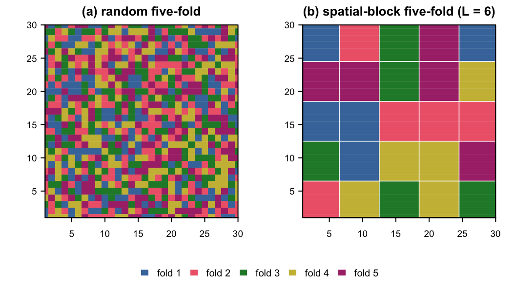
Builds both partitions of the 900 cells — random five-fold (seed 1) and spatial-block five-fold (25 blocks of side 6, whole blocks round-robined to folds after a seed-36 shuffle) — then re-runs the B = 80 selection inside every training fold of both partitions: ten selections in all. The GCF arm of step 3 uses these per-fold sets, so no validation cell ever influences the features it is predicted with.

Code

R — from R/20-sim-cv.R and R/01-helpers.R

fold_sp <- gcf_folds_rr(bid, K = 5L, seed = 36L)   # whole blocks -> folds
fold_rd <- gcf_folds_random(nrow(sim), K = 5L, seed = 1L)

# leakage-safe: one selection per training fold (x2 partitions = 10)
S_sp <- lapply(1:5, function(k)
  gcf::gcf_select(field, y = sim$y1, blocks = bid,
                  train = which(fold_sp != k), B = 80)$selected)

Example output

Demo run fig03 — the two partitions. Random assignment (a) measures interpolation: every validation cell has training neighbours. Spatial-block assignment (b) measures transfer: whole 6 × 6 blocks are held out, so a validation cell's entire neighbourhood is unseen. The paper reports both, and the gap between them is itself informative.

How to read this result

• All ten selections return 8 variables — the same three covariates plus five derived features per fold (results/sim-selected-by-fold.csv). The selection is stable under refolding.
• Per-fold selection keeps the validation leakage-free. Each training fold selects its own features, so validation rows never vote. The ten B = 80 selections are ~80 % of this step's 21 seconds.
• Blocks respect geography, folds respect blocks. Every block lands entirely inside one fold — the property that makes spatial-block CV a test of transfer.

Step 3 · R/30-sim-permodel.R

Simulation — seven learners, base vs GCF (paper Table 2)

What this step does

Runs the paper's per-model comparison: every learner fits twice per fold — once on the three raw covariates, once on that fold's re-selected GCF set — under both partitions. Learner settings are ported verbatim from the paper's engine, and every fit starts from set.seed(1), so each fit is a pure function of its inputs. The finished wide table is then compared byte-for-byte against the published Table 2 shipped in data/paper-tables/.

Code

R — from R/30-sim-permodel.R

X <- as.matrix(field$candidates)     # the paper's engine used a matrix
x_cols <- field$meta$feature[field$meta$category == "X"]

for (ln in LEARNERS) for (pt in c("random", "spatial")) {
  fold <- fold_of[[pt]]; Sb <- S_of[[pt]]
  b <- gcf_cv(X, y, fold, function(k) x_cols, ln)                 # baseline
  g <- gcf_cv(X, y, fold, function(k) Sb[[as.character(k)]], ln)  # GCF
  # per-fold mean/sd of R2 and RMSE + relative improvements -> p1
}
t2 <- gcf_permodel_wide(p1, best)     # the paper's Table-2 shape
compare_with_paper(F_TABLE02, "data/paper-tables/table02-sim-permodel.csv")

Result — Table 2, reproduced byte-for-byte

Learner	Best	Random CV — R²			Random CV — RMSE			Spatial CV — R²			Spatial CV — RMSE
		base	GCF	imp.%	base	GCF	imp.%	base	GCF	imp.%	base	GCF	imp.%
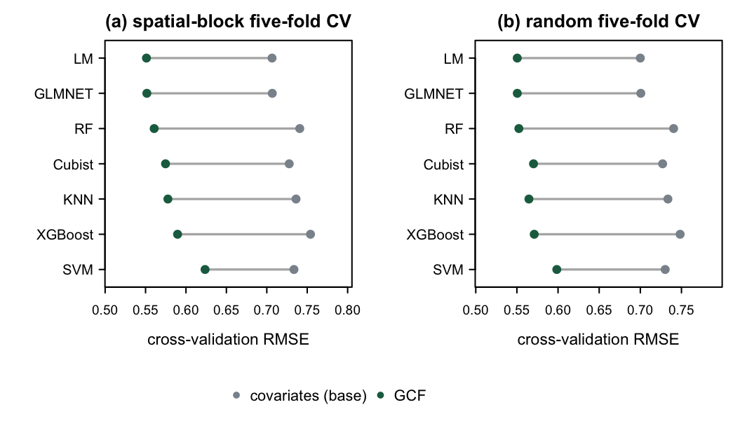
LM	*	0.514	0.700	36.0	0.700	0.550	21.4	0.469	0.668	42.4	0.706	0.551	22.0
GLMNET		0.514	0.700	36.2	0.701	0.550	21.4	0.470	0.668	42.1	0.707	0.552	22.0
RF		0.457	0.697	52.6	0.740	0.552	25.4	0.419	0.657	56.5	0.741	0.561	24.3
Cubist		0.476	0.678	42.3	0.727	0.570	21.6	0.438	0.637	45.6	0.728	0.575	21.0
KNN		0.467	0.684	46.5	0.734	0.565	23.0	0.429	0.637	48.5	0.736	0.578	21.5
XGBoost		0.445	0.677	52.1	0.748	0.571	23.7	0.399	0.619	55.2	0.754	0.590	21.8
SVM		0.472	0.645	36.7	0.730	0.598	18.0	0.433	0.591	36.6	0.734	0.624	15.0

results/table02-sim-permodel.csv — byte-identical to the published Table 2 (results/sim-permodel-check.csv lists all 84 numeric cells side by side; every difference is 0). Learners sorted by spatial GCF RMSE; the asterisk marks the adopted learner. Improvements are relative percentages.

Demo run fig04 — Table 2 as a picture: RMSE of the covariate baseline (grey) and GCF (green) per learner, spatial-block (a) and random (b) CV. Every learner moves left; the linear models move furthest left of all.

Why the match is exact, not approximate

Four links in a chain: (1) the gcf package is a verbatim port of the paper's engine, validated to max|diff| = 0 on ψ, Z_x, candidates and selections; (2) folds use the paper's seeds (36 / 1); (3) every selection re-seeds seed = 1; (4) every learner fit starts from set.seed(1) with the paper's exact settings. Same inputs, same code, same package versions — same bytes.

How to read this result

• All seven learners improve, under both partitions. That pattern — not any single number — is the paper's claim: the gain is attributable to the representation, not to a lucky algorithm.
• GCF-based LM wins. Spatial RMSE 0.551 against 0.706 for baseline LM. The features encode the spatial structure before fitting, so a simple linear map on top suffices — and the baseline's own ordering (LM 0.470 spatial R² vs RF 0.419) shows there was little residual nonlinearity for trees to exploit.
• The spatial gain exceeds the random gain (RF +56.5 % vs +52.6 % R²): neighbourhood features transfer to unseen blocks better than point values do — the property that matters for mapping.

Step 4 · R/40-case-field.R

Case study — real feature generation on the 958 observed cells

What this step does

Runs the identical gcf_field() call the paper uses — 9 buffers from 20 to 100 km, 21 quantile levels, bands {20,30}/{90,100} km, d_norm = 100 — on the 958 observed cells of the SWAFR grid, in about a minute. It generates the paper's Table 4 from the resulting field and then runs one B = 80 stability selection with 132 km blocks.

Code

R — from R/40-case-field.R

obs <- bio_grid[bio_grid$observed, ]           # 958 sampled cells
field <- gcf::gcf_field(obs, coords = c("xkm", "ykm"), vars = CASE_VARS,
                        buffers = seq(20, 100, 10), probs = seq(0, 1, 0.05),
                        d_norm = 100, include_vario_exp = TRUE,
                        vario_buffers = seq(20, 100, 10),
                        fine_band = c(20, 30), broad_band = c(90, 100))
# 958 x 372 candidates; psi 958 x 996; Zx 958 x 2268

bid <- gcf::gcf_blocks(obs[, c("xkm", "ykm")], 132)   # 38 occupied blocks
sel <- gcf::gcf_select(field, y = obs$richness, blocks = bid, B = 80)

Result — Table 4, regenerated byte-for-byte

Category	Symbol	Raw count	Reduced count	Construction
Covariates (x)	x	12	12	raw covariates
Spatial pattern (ψ)	psi	996	240	11 operators, band-averaged
Neighbourhood distribution (Zx)	Zx	2,268	120	5 quantile functionals × 2 scale bands
Total		3,276	372

results/table04-case-predictor-categories.csv — byte-identical to the published Table 4. The counts depend only on the settings (12 covariates × 83 ψ columns; 12 × 9 buffers × 21 quantiles; 12 × (20 P + 10 D) + 12).

Is the expansion worth it? The paper's screening figure

Before any selection or model, the paper asks a simple question of the 3,276 raw predictors: how strongly does each one correlate with richness at the 958 observed cells? The purpose is descriptive — to see whether derived features carry signal beyond the covariates they come from — and it plays no part in the selection, which would otherwise leak the response.

Published reference · GCF Fig. 6 Absolute Pearson correlation with species richness (Song 2026, Figure 6): the twelve original covariates (grey), the spatial pattern features (blue) and the neighbourhood distribution features (orange), each group split by source covariate; every dot is one predictor.

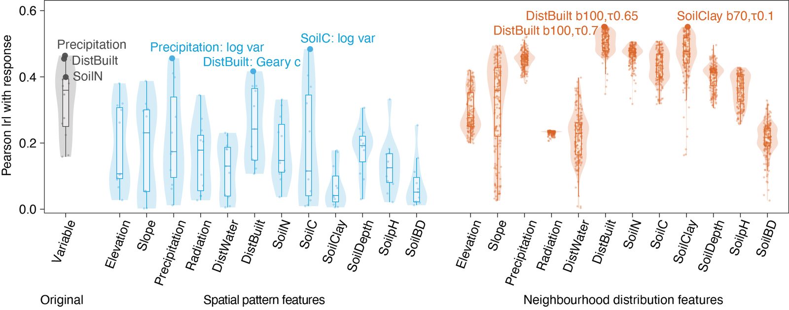
Predictor category	Max |r|	Median |r|	Main influencing factors
Original covariates x	0.464	0.359	Precipitation 0.464, DistBuilt 0.455, SoilN 0.399
Spatial pattern ψ	0.494	≈ 0.13	log local variance of Precipitation 0.494 and of SoilC 0.492
Neighbourhood distribution Zx	0.544	0.348	median of DistBuilt and 10th quantile of SoilClay, both 0.544

Values as reported in the paper's Section 4.2.

How to read this figure

• The best derived features beat the best covariate. The strongest Z_x feature reaches |r| = 0.544, about 17 % above precipitation's 0.464. What surrounds a cell predicts its richness better than what is in it.
• The two families have different shapes. Z_x features are uniformly useful — tight violins, median close to the covariates'. ψ features include a few very strong members — long violins. The selection takes what it needs from each: three ψ features and six Z_x features in the final model.
• A mid-ranked covariate can have the strongest neighbourhood. SoilClay ranks fifth among the covariates at point level (|r| = 0.380 in data/bio-grid.csv), yet its low neighbourhood quantile ties for the strongest predictor of all at 0.544 — and the same functional is one the selection keeps (SoilClay_D_broad_lotail).

What the selection keeps

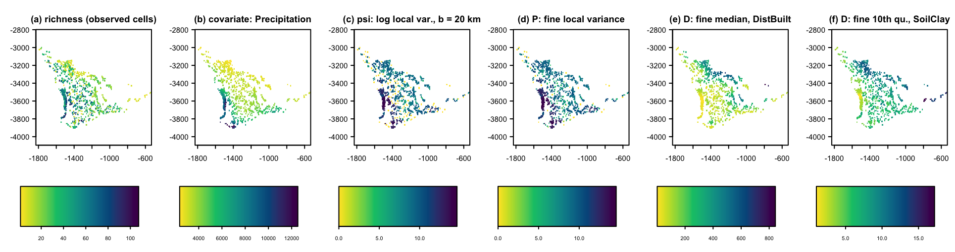
The selection is built around broad-band (90–100 km) context features — Precipitation_D_broad_hitail, DistBuilt_D_broad_med, SoilC_D_broad_iqr, SoilClay_D_broad_lotail, SoilDepth_D_broad_hitail, SoilpH_D_broad_med — together with the pattern feature Slope_P_lvar_broad. They enter the model alongside the twelve covariates, and they are among the nine derived features the paper maps in its Figure 5 (results/case-selected-observed-demo.csv lists the full set with selection frequencies).

Published reference · GCF Fig. 5 The paper's full-support selection, mapped (Song 2026, Figure 5; also shown at the top of this page). (a) The three spatial pattern features: ψ_V of slope and of precipitation, ψ_P of distance to built-up areas. (b) The six neighbourhood distribution features: Z_0.90 of precipitation, Z_0.50 of distance to built-up areas, IQR Z of soil organic carbon, Z_0.10 of soil clay, Z_0.90 of soil depth and Z_0.50 of soil pH — all at the broad 90–100 km band.

Demo run fig05 — the demo field over the observed cells (10 km cells drawn at 14 km for visibility; axes are EPSG:3577 Albers km): observed richness (a), the strongest covariate precipitation (b), its ψ log local variance at the 20 km buffer (c), the fine-band pattern candidate built from it (d), and two fine-band context candidates — the median of distance to built areas (e) and the 10th quantile of soil clay (f). The paper's selection keeps the broad-band (90–100 km) versions of both functionals, mapped in its Figure 5 at the top of this page.

For your own data

Build the field on every location you will ever predict — sampled and unsampled together (§2.3, rule 1) — then run the selection and the learner on the sampled rows. The numbers the paper reports come from the field built on the full 6,229-cell grid, stored inside case_final.rds.

Step 5 · R/50-case-tables.R

Case study — Tables 5, 6 and 7

What this step does

Reads data/case_final.rds — the paper's computed four-part validation, shipped with the code — and turns it into the paper's three case tables with the paper's own formatting code (the same gcf_permodel_wide(), renames and rounding). The step takes under a second, and each CSV is byte-identical to the published table.

The validation design behind the tables

Published reference · GCF Fig. 7 The two cross-validation schemes of the case study (Song 2026, Figure 7). (a) Random folds, about 192 cells each: every validation cell has training cells next to it, so this measures interpolation. (b) The variogram of richness after removing the covariate trend levels off at a range of 66 km — beyond that distance, residuals are no longer spatially dependent. (c) Spatial-block folds: 38 occupied blocks of side L = 2 × 66 = 132 km are assigned whole to folds, so a validation cell's short-range neighbours are never in training. 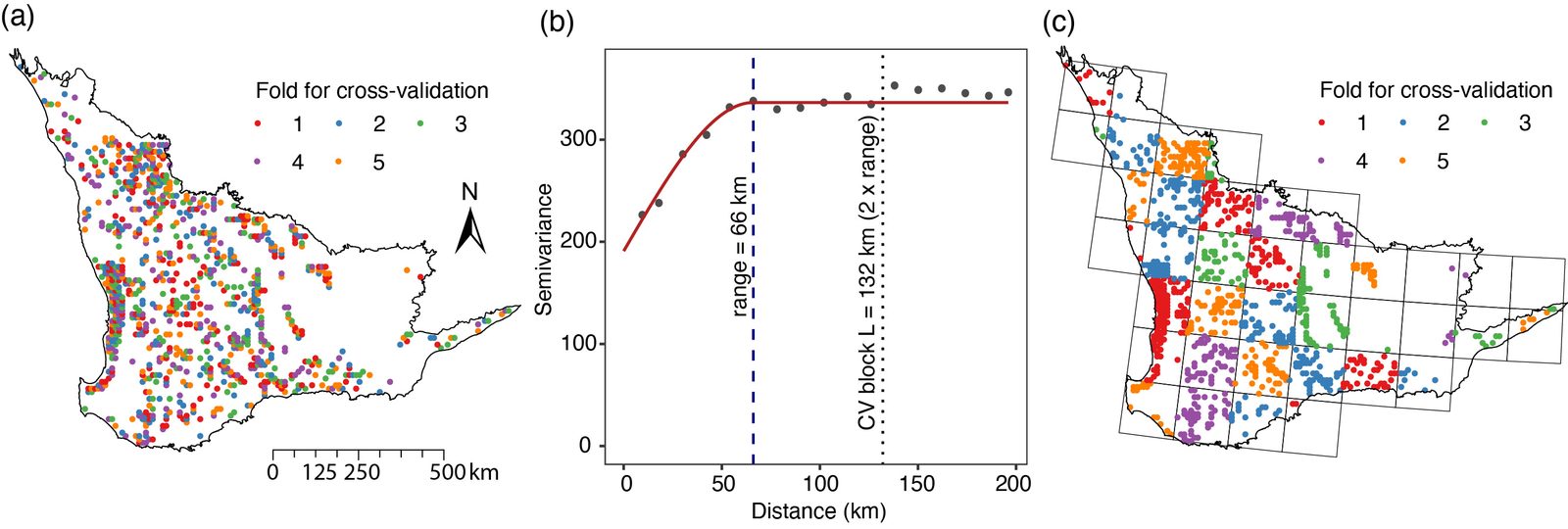This is the case-study counterpart of demo fig03, and the reason CASE_L is 132.

Result — Table 5 (per-model, case)

Learner	Best	Random CV — R²			Random CV — RMSE			Spatial CV — R²			Spatial CV — RMSE
		base	GCF	imp.%	base	GCF	imp.%	base	GCF	imp.%	base	GCF	imp.%
RF	*	0.441	0.444	0.7	17.114	17.043	0.4	0.296	0.346	16.7	17.966	17.428	3.0
Cubist		0.431	0.435	0.9	17.230	17.181	0.3	0.283	0.342	21.1	18.065	17.506	3.1
KNN		0.427	0.432	1.3	17.321	17.232	0.5	0.296	0.320	8.2	18.039	17.743	1.6
XGBoost		0.401	0.428	6.9	17.704	17.291	2.3	0.261	0.315	20.3	18.304	17.795	2.8
SVM		0.398	0.419	5.4	17.750	17.418	1.9	0.275	0.327	18.6	18.489	17.849	3.5
GLMNET		0.350	0.393	12.3	18.451	17.822	3.4	0.259	0.302	16.9	18.575	18.054	2.8
LM		0.349	0.395	13.2	18.464	17.801	3.6	0.253	0.286	13.0	18.647	18.279	2.0

results/table05-case-permodel.csv — byte-identical to the published Table 5. All seven learners improve under both partitions; RF is adopted (smallest spatial GCF RMSE). Spatial-block R² improvements run from 8.2 % (KNN) to 21.1 % (Cubist).

Result — Tables 6 and 7 (feature sets and Shapley)

Feature set	R²	sd	RMSE	sd	ΔR²%	ΔRMSE%
x	0.296	0.142	17.966	2.138	0	0
x+ψ	0.337	0.112	17.500	2.187	13.7	2.6
x+Zx	0.329	0.119	17.613	2.415	11.2	2.0
GCF (x+ψ+Zx)	0.346	0.108	17.428	2.497	16.7	3.0

Table 6 (results/table06-case-featuresets.csv, byte-identical) — RF, spatial-block CV, per-fold selected sets decomposed by category.

Category	Shapley φ	Share	Total R²
x (covariates)	0.158	0.456	0.346
ψ (spatial pattern)	0.086	0.248
Zx (neighbourhood distribution)	0.102	0.296

Table 7 (results/table07-case-shapley.csv, byte-identical) — exact three-player Shapley decomposition of the spatial-block R²; the three φ values sum to the GCF total by construction.

How to read this result

• The two families are complementary. GCF (0.346) beats both x+ψ (0.337) and x+Z_x (0.329) — neither family alone accounts for the full gain. The attribution file (results/case-attribution.csv: gain_P 2.594, gain_D 1.965, gain_full 2.999, shared −1.560) says the same in RMSE terms: the families overlap partly, and the joint gain exceeds either alone.
• Together the derived features carry 54 % of the explained variance (Shapley shares 0.248 + 0.296) — on a study where the 12 covariates were chosen by experts precisely for their predictive value.
• The gain is largest under spatial blocks (RF +16.7 % R², against +0.7 % under random folds). The neighbourhood features earn their keep where mapping needs them — predicting unseen blocks.

The paper's robustness analyses

The third part of the paper's validation asks when the gain holds and when it grows. Three conditions that make real mapping hard are imposed in turn: fewer training samples, whole regions withheld, and covariates taken away. The results sit in case_final.rds as regA–regC ; the figure and numbers below are the paper's.

Published reference · GCF Fig. 8 Robustness of the GCF gain (Song 2026, Figure 8). (a) RMSE gain (covariate-only RF minus GCF) by training fraction ρ; point size is the between-fold sd. (b) The west–central–east split and (c) RMSE when each region is withheld entirely. (d) RMSE and (e) accuracy recovery rate as the strongest covariates are removed first, from k = 12 down to k = 1. ARR = (RMSE_mean − RMSE(k)) / (RMSE_mean − RMSE_k=12), where RMSE_mean = sd(y) is the error of predicting the global mean.

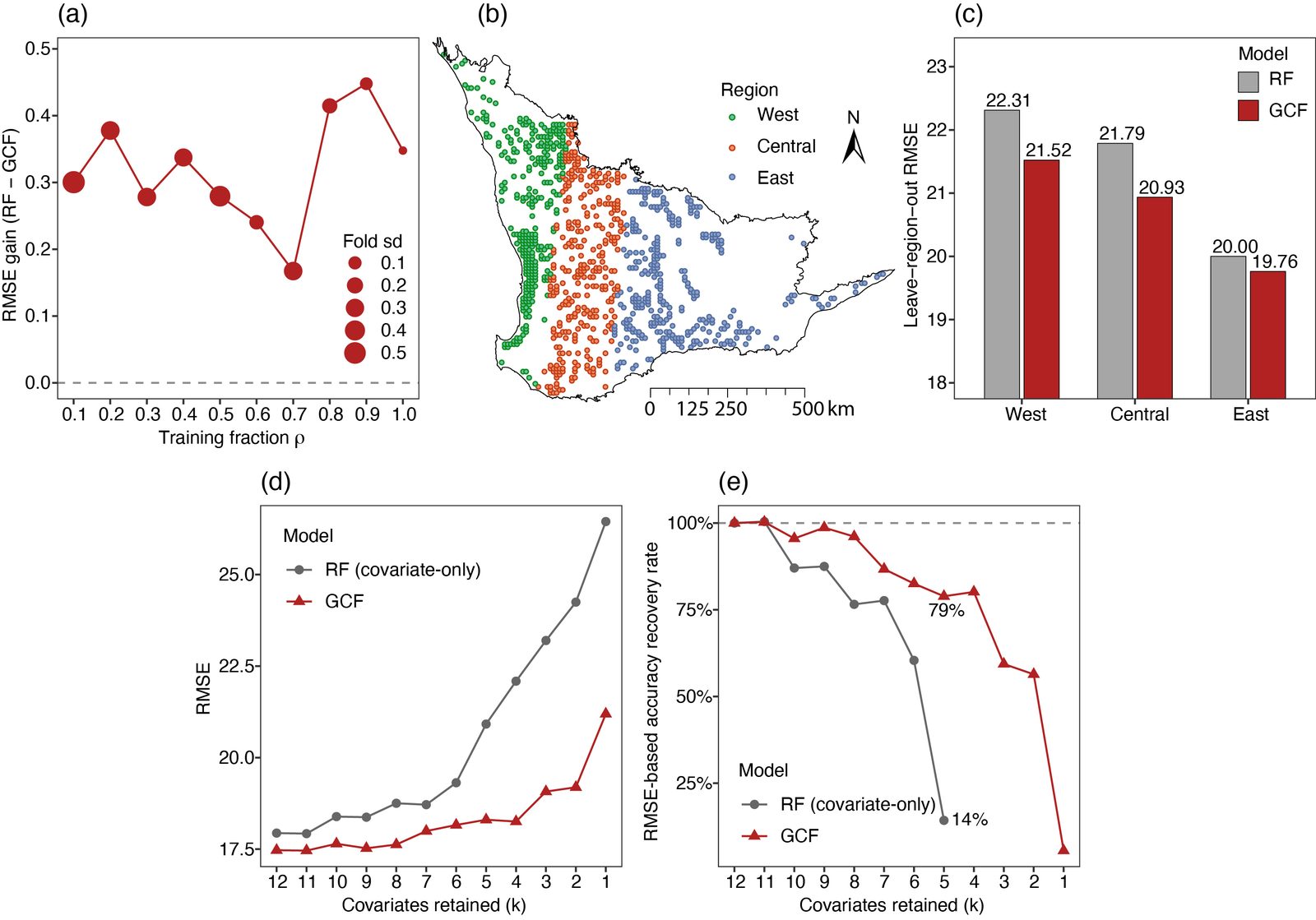
Stress	Setting	Covariate-only RF	GCF	Reading
Sparse sampling	training fraction ρ = 0.1	RMSE gain 0.30		the gain is positive at every ρ, and the between-fold spread shrinks as training data grow
	training fraction ρ = 0.9	RMSE gain 0.45
Spatial extrapolation (leave-region-out RMSE)	West withheld	22.31	21.52	GCF is lower in all three regions (gains 0.79, 0.85 and 0.24)
	Central withheld	21.79	20.93
	East withheld	20.00	19.76
Covariate scarcity (strongest removed first)	k = 5 covariates kept: ARR	14 %	79 %	GCF loses accuracy gradually and keeps R² positive throughout
	k = 1 covariate kept: RMSE increase	+47 %	+21 %

Key numbers of the three robustness analyses, from the paper's Section 4.3 and the bar labels of its Figure 8(c).

How to read this result

• Covariate scarcity is where GCF matters most. With seven of twelve covariates removed, covariate-only RF has lost 86 % of what its covariates bought over predicting the mean; GCF has lost 21 %. The neighbourhoods of the remaining covariates still describe the geographical setting that the removed ones measured directly. For data-poor regions this is the practical case for the method.
• The gain transfers to whole withheld regions. Withholding a region is a harder test than spatial blocks, and GCF wins in all three — west, central and east.
• The gain holds with few samples. Feature construction uses the covariates at all 6,229 cells, not the response, so it is unaffected by how many cells are sampled.

Step 6 · R/60-case-prediction.R

Case study — the two prediction surfaces

What this step does

Maps the paper's Part-4 result: RF trained on all 958 observed cells — once on the covariates, once on the 21-variable full-support GCF set — predicting all 6,229 grid cells. Both finished surfaces live in case_final$prediction; this step reads and draws them, the difference, and the paper's west–east cross-section.

Example output

Demo run fig06 — predicted species richness from GCF-RF (a) and covariate-RF (b) on a shared scale; their difference (c; blue = GCF higher, scale clipped at the 98th percentile of |difference|); and the cross-section at y = −3654 km (d), the paper's transect. Axes are EPSG:3577 Albers km (the paper's own maps use a Web-Mercator display projection; the values are identical).

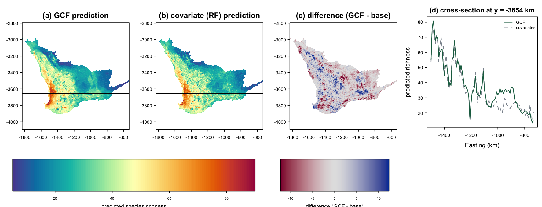
Surface	Mean	sd	Min	Max	Note
GCF prediction	33.211	15.362	5.164	90.002
covariate (RF) prediction	33.566	14.603	6.689	88.508	r(GCF, base) = 0.953
difference (GCF − base)	−0.355	4.649	−21.714	16.607	GCF higher in 44.4 % of cells

results/case-prediction-summary.csv. The two surfaces agree on the broad gradient (r = 0.953) and disagree exactly where neighbourhood information matters — the difference map is spatially organised, not noise.

The published prediction figure

The paper's purpose in this last part is to judge the map itself, not only its cross-validated error: a surface used for conservation planning should keep real contrasts and avoid cell-to-cell speckle. Besides the two surfaces and transects, the paper therefore maps the local variance V_ℓ of each prediction — the variance of predicted values within each cell's neighbourhood — which demo fig06 does not draw.

Published reference · GCF Fig. 9 Spatial prediction of species richness (Song 2026, Figure 9). (a) GCF-based RF and (b) covariate-only RF predictions, with the two transect lines; (c) both predictions along x = −1506 km and y = −3654 km; (d, e) local variance V_ℓ of each prediction; (f) the difference ΔV_ℓ (GCF − RF), blue where GCF is locally smoother. Panels (a), (b) and the y-transect of (c) are the content of demo fig06, drawn from the same stored surfaces.

How to read this result

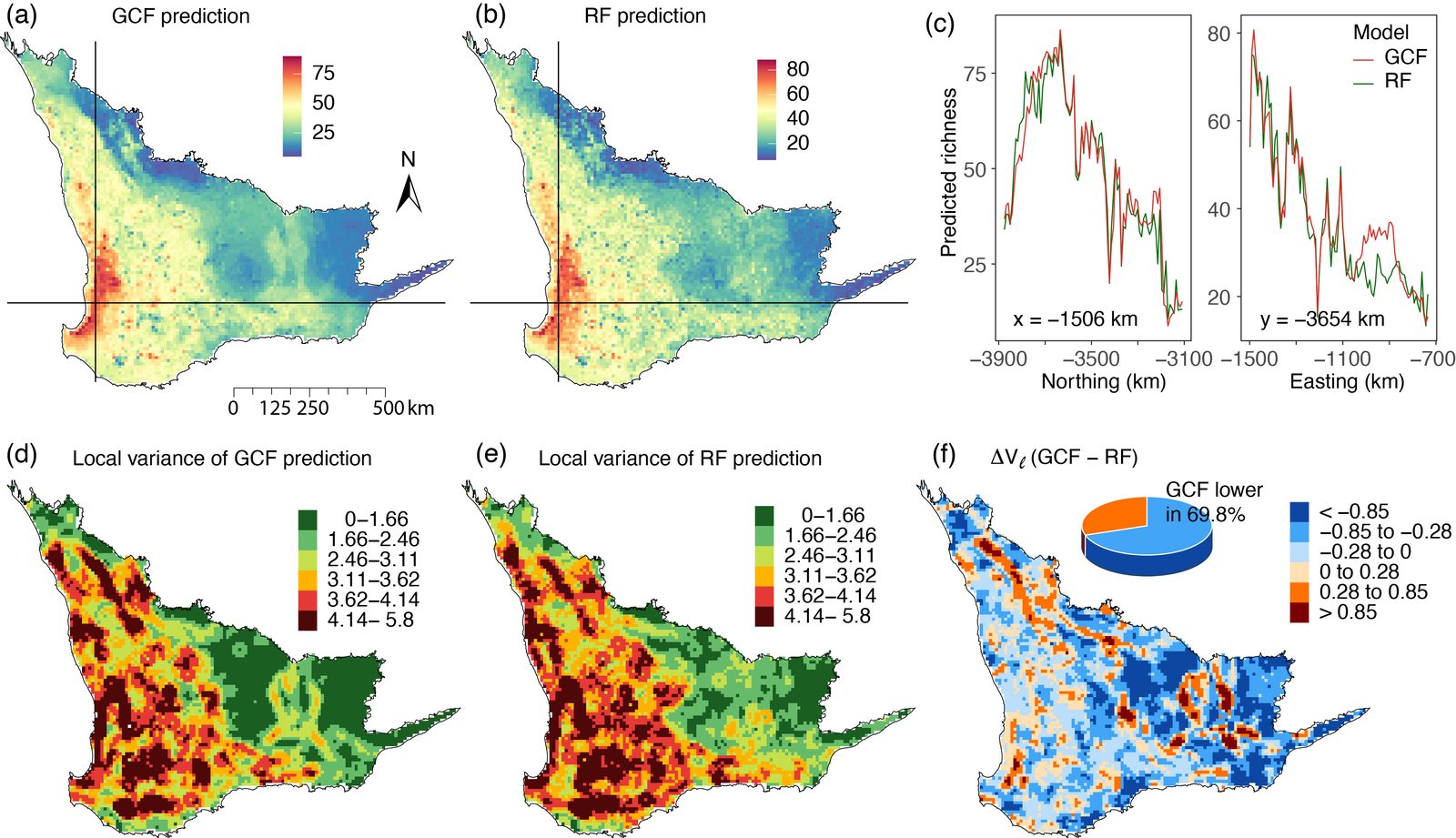
• Follow the transect. Along y = −3654 km the GCF surface keeps the high peaks (up to ~80) and the deep troughs that the covariate-only surface dampens — richer features let the learner commit to local extremes instead of hedging towards the regional mean.
• The GCF surface has slightly larger spread (sd 15.36 vs 14.60) with the same mean level — consistent with preserved contrasts rather than added noise, given its lower cross-validated error in Table 5.
• Smoother locally, sharper regionally. In the paper's panel (f), GCF has the lower local variance over 69.8 % of the region: less cell-to-cell speckle, more coherent transitions. That does not contradict the larger overall spread — the two measure different scales. Neighbourhood features change slowly from cell to cell, so they steady the prediction locally while still separating high-richness from low-richness areas. On the y-transect of panel (c), east of about −1100 km, GCF holds a plateau near 35 where covariate-only RF drops towards 25 and fluctuates.
• The difference map is the sampling map's shadow. The largest disagreements sit in the sparsely observed east and interior — where a validation block has few nearby samples and the neighbourhood features carry the most extra information.

3.3 Reading the Results Together

4 Adaptation, Writing & Reproducibility

4.1 Port to Your Domain

GCF applies wherever you have a response measured at some locations and covariates measured over a grid or a dense point set with projected coordinates: soil properties, air quality, species richness, urban indicators, mineral prospectivity. The whole method is two calls:

library(gcf)
field <- gcf_field(mydata, coords = c("xkm", "ykm"),
                   vars = my_covariates,
                   buffers = my_buffers,          # e.g. 1-5 cell diameters
                   fine_band = head(my_buffers, 2),
                   broad_band = tail(my_buffers, 2))
blocks <- gcf_blocks(mydata[, c("xkm", "ykm")], size = 2 * variogram_range)
sel <- gcf_select(field, y = mydata$y[train], blocks = blocks, train = train)
X <- as.matrix(field$candidates)[, sel$selected]   # -> any learner

What to edit

1. config/project-config.R — coordinates, response, covariates (CASE_* block), then the spatial settings below. Nothing else.
2. *_BUFFERS — a series from roughly one cell diameter up to at or beyond the response's variogram range. Integer values (§2.3, rule 3).
3. *_FINE / *_BROAD — the two ends of your buffer series; the defaults (min / max buffer) are a sensible start.
4. *_L — spatial-block side ≈ 2 × the residual variogram range, so validation blocks sit beyond short-range dependence. Fit a variogram to the covariate-detrended response to get the range, as the paper does.
5. Selection settings (SEL_*) — the paper's B = 80, 0.7, π = 0.6, K = 20 travel well; lower B while iterating, restore it for the run you report.
6. Nothing else. Run Rscript run-all.R.

Choosing what to expand

• Every covariate must exist at the prediction locations — features are computed there too. Remote-sensing, terrain, climate and distance-to-feature layers are ideal.
• Give the field the full support once. Build features on observed + prediction locations together, in one call, then subset rows for training.
• Let the selection do the pruning. The candidate field is deliberately generous (31 candidates per covariate); the stability selection with group voting is the part designed for exactly that, so no manual pre-screening is needed.
• Match the buffers to the process scale. Choose a buffer series that straddles the variogram range of the response.

4.2 Write the Paper

The published study has a clean architecture worth copying: define the feature families, prove the mechanism on a simulation, then validate on the real case with a per-model table, a feature-set decomposition, and prediction surfaces.

Manuscript skeleton

1  Introduction        — spatial prediction constrained by heterogeneity and
                          sparse sampling; methods grow model complexity while
                          underusing the covariates' own spatial structure (aims)
2  Generalized covariate field
                        — 2.1 spatial pattern features (11 operators x buffers)
                          2.2 neighbourhood distribution features (quantiles)
                          2.3 functional reduction (bands; D and P candidates)
                          2.4 selection: rf_imp + block stability + group voting
                          2.5 validation: dual five-fold CV, L = 2 x range
3  Simulation          — design; per-model table; why linear learners win
4  Case study          — data; the field (Table-4 shape); selection;
                          per-model table; feature sets + Shapley; prediction
5  Discussion          — representation vs model complexity; transfer gains;
                          support and scale choices
6  Conclusions         — 6-8 sentences answering the aims

4.3 Final Reproducibility Package

What is in the download, and what is not

References & credits

Demo outputs were generated by the scripts in this folder using the gcf package and its bundled data; the case-study validation tables and surfaces come from the paper's computed result object, shipped here unchanged.

1. Song Y (2026). Generalized covariate field (GCF): spatial-pattern and neighbourhood-distribution feature expansion improves geospatial prediction. International Journal of Geographical Information Science 40:1–29. doi:10.1080/13658816.2026.2729719 · PDF (source of the method and of every published number on this page)
2. Song Y (2026). gcf: Generalized Covariate Field. R package version 0.1.0. CRAN.R-project.org/package=gcf, doi:10.32614/CRAN.package.gcf (the reference implementation — a verbatim, validated port of the paper's analysis engine — and the source of both data sets)
3. GCF code, data and examples — github.com/yongzesong/gcf (the standalone R implementation gcf.R, the simulation data and a worked example, as published with the paper)
4. Mokany K, McCarthy JK, Falster DS, Gallagher RV, Harwood TD, Kooyman R, Westoby M (2022). Patterns and drivers of plant diversity across Australia. Ecography 2022(11):e06426. doi:10.1111/ecog.06426 (the vascular-plant richness observations behind the case study)
5. Online GCF calculator — yongzesong.com/app/gcf/ (the same gcf feature engine compiled to WebAssembly, running entirely in the browser)