Spatial information explained
Song, Y. (2026). Spatial information explained by prediction models under block cross-validation. ISPRS Journal of Photogrammetry and Remote Sensing, 242, 984–1000. https://doi.org/10.1016/j.isprsjprs.2026.09.034
Full text · BibTeX · Code · TutorialSpatial information explained (SIE) is a validation metric for spatial prediction models that quantifies how much of the spatial information in a response variable a model explains, as the relative reduction in spatial information from the response to the prediction residuals.[1] It was introduced by Yongze Song in 2026 in the ISPRS Journal of Photogrammetry and Remote Sensing, in a special issue entitled XGeoAI. SIE is intended to complement accuracy metrics such as the root mean squared error (RMSE) and the coefficient of determination (R2), which quantify prediction error but not the spatial structure a model captures.
SIE measures spatial information as the mutual information between a variable and its spatial location, estimated after discretizing values into equal-frequency bins and locations into a regular grid. Residuals are taken from out-of-fold predictions of spatial block cross-validation, which separates training and evaluation data in space. Scale-specific values computed at several grid resolutions are combined into a multi-scale SIE with softmax weights derived from the spatial information of the response, so that no resolution needs to be selected.[1] SIE ranges from 0, when a model does not reduce the spatial information of the response, to 1, when the residuals retain none.
In a case study predicting C4 natural grass area across Australia with ten machine learning models, the k-nearest neighbour model, a neural network and XGBoost reached the highest multi-scale SIE of about 0.50, while support vector regression had the highest accuracy. SIE rankings differed from accuracy rankings, and random cross-validation overstated SIE relative to block cross-validation for all ten models, by 2.1–17.0%.[1]
Background
Spatial validation governs both the training and the evaluation of geospatial prediction models, from spatial statistics to geospatial artificial intelligence, and informs the choice among competing models.[2] Research on spatial validation addresses the metrics used to quantify performance, the cross-validation designs used to partition data, and the effects of spatial features of the data on validation outcomes. Block cross-validation partitions the study area into contiguous blocks so that spatially proximate observations do not appear in both training and test sets, reducing the optimistic bias of random cross-validation when samples are spatially dependent.[3][4]
Existing validation methods fall into three groups: global accuracy and error metrics such as RMSE, mean absolute error and R2; spatial explainability methods such as Shapley additive explanations and GeoShapley, which attribute predictions to predictors and to location;[14] and methods based on the spatial structure of residuals. The last group rests on the principle that a well-performing spatial model leaves spatially random residuals. Moran's I of residuals detects remaining spatial autocorrelation,[13] the degree of spatial interpretability measures the share of spatially stratified variance a model explains,[5] and geocomplexity-based diagnostics relate errors to the complexity of local spatial patterns.[8]
The paper identifies three gaps that SIE was designed to address: existing spatial validation metrics are computed under random cross-validation, and none is designed for block cross-validation; there was no formal measure of the quantity of spatial information in spatial data; and no metric quantified the total spatial information a model explains across the range of scales at which spatial dependence operates.[1] Mutual information, a nonparametric measure of statistical dependence that has been used in geographic information science to characterize spatial association and stratification,[9] provides the measure of spatial information on which SIE is built.
Definition
Spatial information
Let Y be a spatially distributed variable and S its spatial location, represented by spatial units. With H(Y) the Shannon entropy of Y, the spatial information in Y is the reduction in its uncertainty attributable to location:[1]
where H(Y | S) is the uncertainty that remains once the spatial unit is known. A strongly autocorrelated variable carries high spatial information, because location is predictive of value; a spatially random variable carries none. The ratio θ(Y) = I(Y; S) / H(Y) expresses spatial information as a share of total entropy. Because I(Y; S) requires a partition of space, it is a scale-indexed statistic rather than an intrinsic property of a dataset: it generally increases as the partition is refined, approaching H(Y) when each unit holds a single observation, so values from different resolutions are not directly comparable.
The SIE metric
For a model with predictions Ŷ and residuals ε = Y − Ŷ, the residual spatial information I(ε; S) measures the spatial structure left unexplained. SIE is defined as
E = 1 indicates that the residuals contain no remaining spatial information; E = 0 indicates no reduction relative to the response. The upper bound holds because mutual information is non-negative. Values below zero, which arise when the residuals carry more spatial information than the response, are set to zero and taken to indicate model misspecification. Because mutual information is not additive, E measures a relative reduction in the location dependence of the analysed variable rather than a partition of a fixed quantity of information between model and residuals.[1]
Discretization and estimation
Mutual information is estimated from discretized data. Y and ε are each divided into nb equal-frequency bins at their empirical quantiles, which keeps the entropy estimates robust to skewed distributions. The two coordinates are discretized jointly by laying a regular grid over the spatial extent of the data and assigning each observation the label of its cell, so that S encodes position in both dimensions. Entropy and mutual information are then computed from the empirical distributions, in nats:
which is algebraically equivalent to the entropy-based definition. Under equal-frequency binning H(Y) ≈ log nb. The plug-in estimate carries a positive bias whose leading term is (nb − 1)(ns − 1) / 2n, where ns is the number of occupied spatial cells and n the number of observations.[10][11] Because the same bias enters both mutual informations and I(ε; S) < I(Y; S), it biases E downwards, making the metric conservative; at a fixed resolution the bias is common to all models and does not alter their ranking.
Residuals from block cross-validation
Residuals of a model fitted to the full dataset would overstate SIE, because spatial autocorrelation lets training observations inform predictions at nearby locations. SIE therefore uses k-fold spatial block cross-validation: the domain is divided into contiguous blocks that are randomly assigned to folds, each fold is predicted by a model trained on the others, and the out-of-fold predictions ŶOOF are concatenated over all folds. The residuals εblock = Y − ŶOOF give a spatially honest estimate, and accuracy metrics computed from the same predictions provide a directly comparable baseline.[1]
Multi-scale SIE
Because spatial dependence operates at several scales, scale-specific SIE Er = 1 − Ir(ε; S) / Ir(Y; S) is computed at a set of grid resolutions r1, …, rK and aggregated as
This discrete form follows from a continuous definition as a weighted integral of Er over a bounded range of resolutions, from the resolution of the observations to the extent of the study area. Scales at which the response carries more spatial information receive larger weights. The softmax may be written with a temperature τ, which the paper fixes at 1 so that the metric has no tunable parameter. Because the weights depend on Y alone, they are the same for every model; selecting the resolution that maximizes Er would instead introduce an upward selection bias. A single resolution is the special case K = 1, and the scale-specific values remain available as a diagnostic profile.[1]
Properties
- Beyond variance and autocorrelation. Mutual information detects systematic differences between the distribution within spatial cells and the overall distribution, including differences in central tendency, dispersion and shape such as skewness or tails. Residuals with a constant conditional mean but spatially varying variance leave residual autocorrelation near zero, while I(ε; S) remains positive.[1]
- Finite-sample ceiling. Even for spatially random residuals the plug-in estimate of I(ε; S) is positive, so E stays below 1 under full learning; the ceiling depends on the number of bins, the grid and the sample size.
- Comparability. E values should be compared across models only under identical discretization settings and sample sizes, with the leading bias term kept small relative to I(Y; S).
- Joint reading with accuracy. Spatially unstructured noise in the predictions can weaken the dependence of residuals on location while increasing error. The paper therefore recommends interpreting E together with accuracy computed under the same validation: higher E with equal or better accuracy indicates stronger spatial learning, whereas higher E with lower accuracy reflects noise effects.[1]
- Weight profile. The shape of the softmax weights is informative: a strongly peaked profile indicates spatial information concentrated at one grain, a near-uniform profile information spread over several scales.
Worked example
A 4 × 4 grid illustrates the calculation. The response is a left-to-right gradient plus a perturbation unrelated to location, Y(i, j) = j + o(i, j) with o ∈ {0, 0.2, 0.4, 0.6}, so that the two equal-frequency bins of Y coincide with the left and right halves of the grid. With nb = 2 bins and a 2 × 2 grid, every cell is pure in the bin of Y, giving I(Y; S) = ln 2.
| Model | Residual bins per cell | I(ε; S) | E |
|---|---|---|---|
| Learns the gradient (Ŷ = j) | 2 low, 2 high in every cell | 0 | 1 |
| Partial learner | 3 : 1 in every cell | ¾ ln 3 − ln 2 = 0.131 | 0.811 |
| No model (Ŷ = 0) | as Y: pure cells | ln 2 = 0.693 | 0 |
Hand calculation, reproduced by the sie.R functions in the tutorial. On a 4 × 4 grid with one observation per cell every cell is trivially pure, I(Y; S) = I(ε; S) for any model and E = 0, which illustrates why grids must be coarse enough for the bias term to stay small.
Evaluation
Simulation study
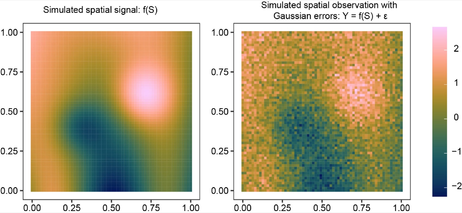
The simulation generated a spatial signal f(S) from five spatial components on the unit square, with observations Y = f(S) + ε under Gaussian noise (Figure 1), and varied only the prediction to represent increasing spatial learning, with 20 bins and an 8 × 8 grid.[1]
| Scenario | Prediction Ŷ | I(Y; S) | I(ε; S) | E |
|---|---|---|---|---|
| No spatial structure | 0 | 0.153 | 0.153 | 0.000 |
| Spatial structure, no model | 0 | 0.778 | 0.778 | 0.000 |
| Partial, 20% | 0.2 f(S) | 0.778 | 0.665 | 0.146 |
| Partial, 50% | 0.5 f(S) | 0.778 | 0.448 | 0.424 |
| Partial, 80% | 0.8 f(S) | 0.778 | 0.229 | 0.705 |
| Full learning | f(S) | 0.778 | 0.154 | 0.802 |
Source: Song (2026), Table 2.
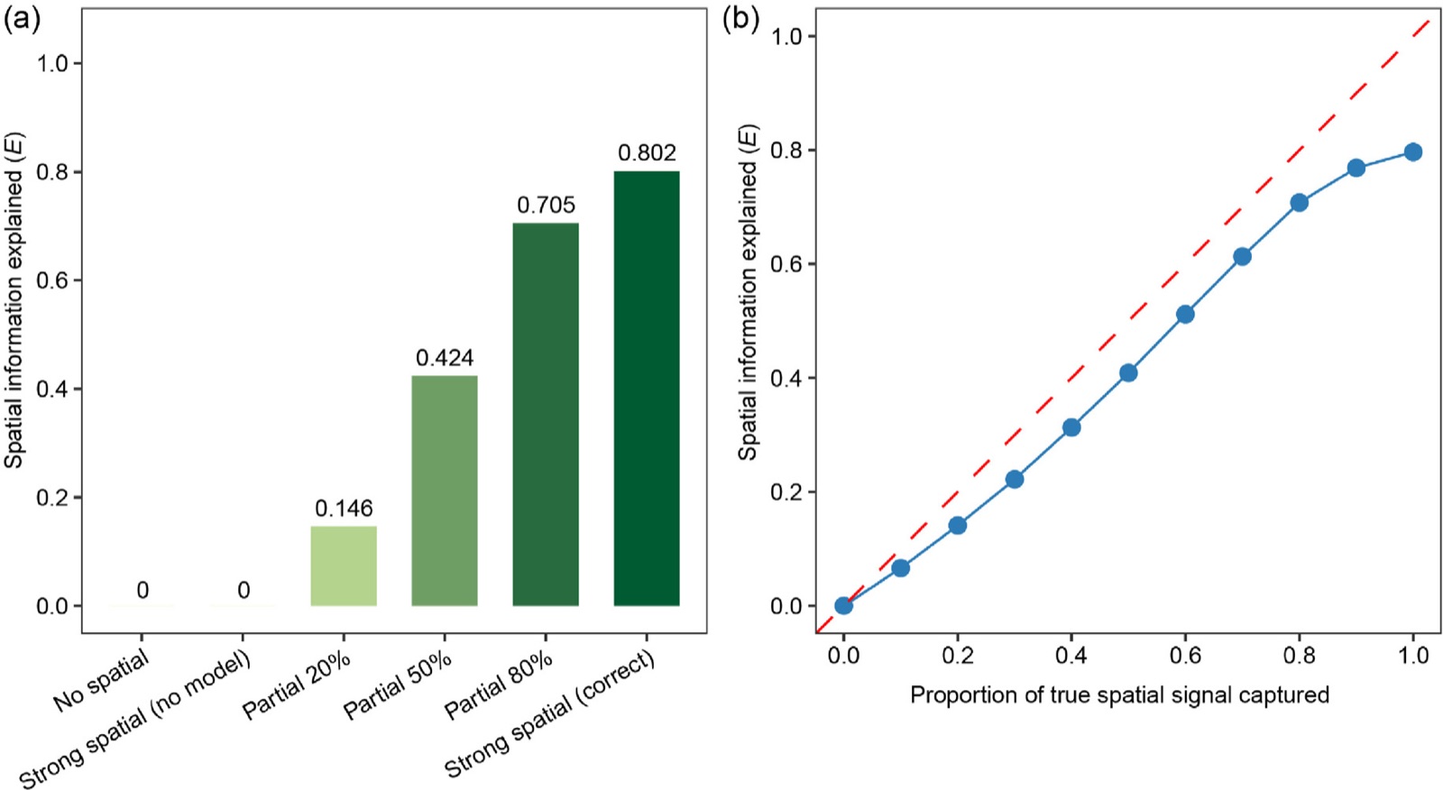
E was zero both without spatial structure and when structure was present but unmodelled, and increased monotonically with the learned proportion, though not proportionally, since mutual information is a nonlinear functional of the joint distribution (Figure 2). The value of 0.802 under full learning reflects the finite-sample noise floor of the estimator: with purely random residuals the estimate of I(ε; S) was still 0.154 nats, close to the 0.153 of the no-structure scenario. Residual maps showed spatial structure decreasing progressively as E rose.
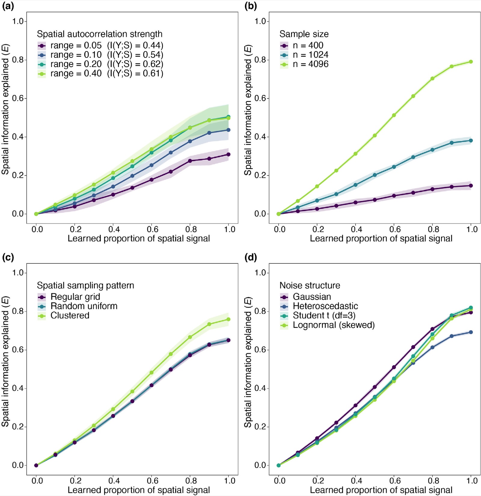
Robustness was examined in 14 configurations across four families, with 20 replicates each: autocorrelation strength (Gaussian random fields with exponential covariance and ranges 0.05–0.40), sample size (400, 1,024 and 4,096), sampling pattern (regular, uniform random, clustered) and noise type (Gaussian, heteroscedastic, Student t, lognormal). E increased monotonically with learning in every configuration (Figure 3). Smaller samples compressed the response — full-learning E fell from 0.79 to 0.38 and 0.15 as the leading bias term rose from 0.15 to 0.58 and 1.50 nats — and heteroscedastic noise lowered the ceiling to 0.69, which the paper attributes to genuine residual spatial structure, since location-dependent dispersion cannot be removed by a conditional-mean prediction.[1]
Case study: C4 grass area in Australia
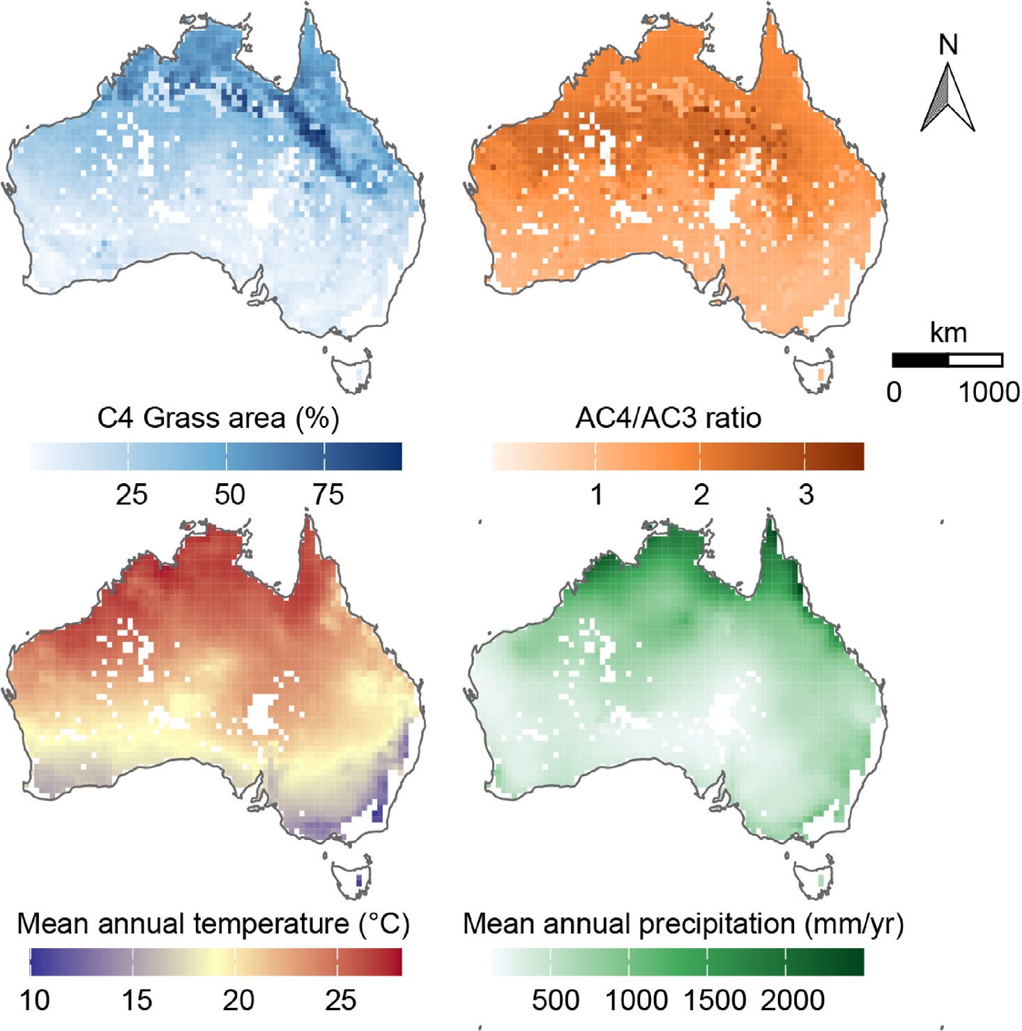
The application evaluated ten machine learning models predicting the percentage of land covered by C4 natural grasses across Australia in 2019, on 2,480 cells of 0.5°, from three predictors: the AC4/AC3 photosynthetic advantage ratio, mean annual temperature and mean annual precipitation (Figure 4).[12] The models spanned four classes — tree ensembles (random forest, XGBoost, LightGBM, gradient boosting), smooth nonlinear models (support vector regression, a neural network averaged over five initializations), an instance-based model (k-nearest neighbours) and linear and spline models (elastic net, lasso, MARS) — with fixed regularized hyperparameters. SIE used five-fold block cross-validation on a 10 × 10 block grid with blocks of about 360 km, 20 bins, and four grids of 900, 600, 450 and 360 km cells.
The response carried 1.071 nats of spatial information at the 360 km grid, so that location accounted for about 36% of its entropy at that grain. All ten models left positive residual spatial information, from 0.646 nats (XGBoost) to 0.840 (lasso). The softmax weights were nearly uniform (0.199 at 900 km to 0.298 at 360 km), indicating spatial information spread across the examined scales; replacing them by linear or uniform weights changed E by less than 0.013 and left the ranking unchanged. Scale-specific Er declined from the coarsest to the finest grid for every model, with a consistent model ordering (Figure 5).[1]
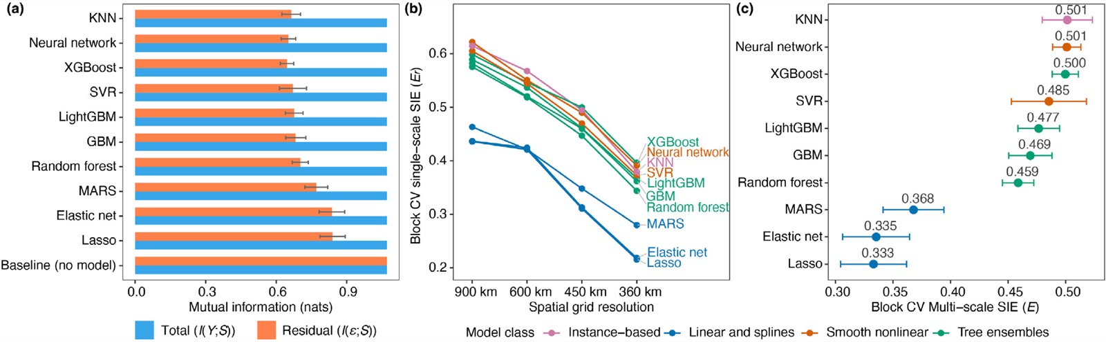
| Model | Class | Multi-scale E | RMSE | R2 | Random CV E |
|---|---|---|---|---|---|
| KNN | Instance-based | 0.501 | 9.23 | 0.727 | 0.554 |
| Neural network | Smooth nonlinear | 0.501 | 8.83 | 0.751 | 0.555 |
| XGBoost | Tree ensemble | 0.500 | 9.21 | 0.729 | 0.558 |
| SVR | Smooth nonlinear | 0.485 | 8.26 | 0.789 | 0.534 |
| LightGBM | Tree ensemble | 0.477 | 9.49 | 0.714 | 0.548 |
| GBM | Tree ensemble | 0.469 | 8.85 | 0.751 | 0.549 |
| Random forest | Tree ensemble | 0.459 | 8.70 | 0.762 | 0.519 |
| MARS | Linear and splines | 0.368 | 9.17 | 0.726 | 0.393 |
| Elastic net | Linear and splines | 0.335 | 9.75 | 0.696 | 0.342 |
| Lasso | Linear and splines | 0.333 | 9.75 | 0.696 | 0.340 |
Source: Song (2026) and the published code (github.com/yongzesong/SIE). RMSE and R2 = 1 − SSE/SST are computed within each held-out fold and averaged over the five folds.
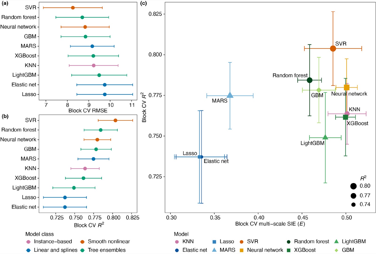
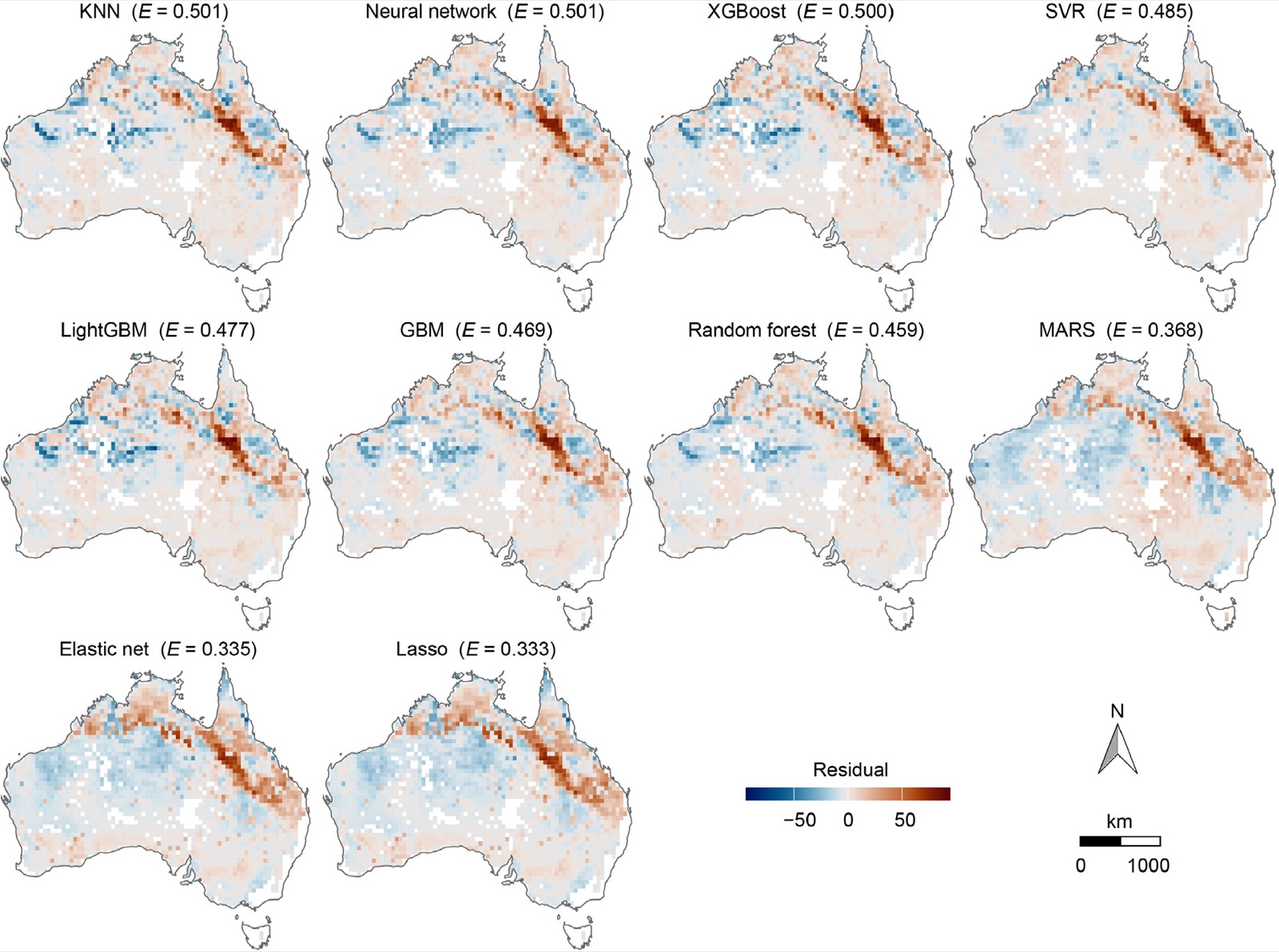
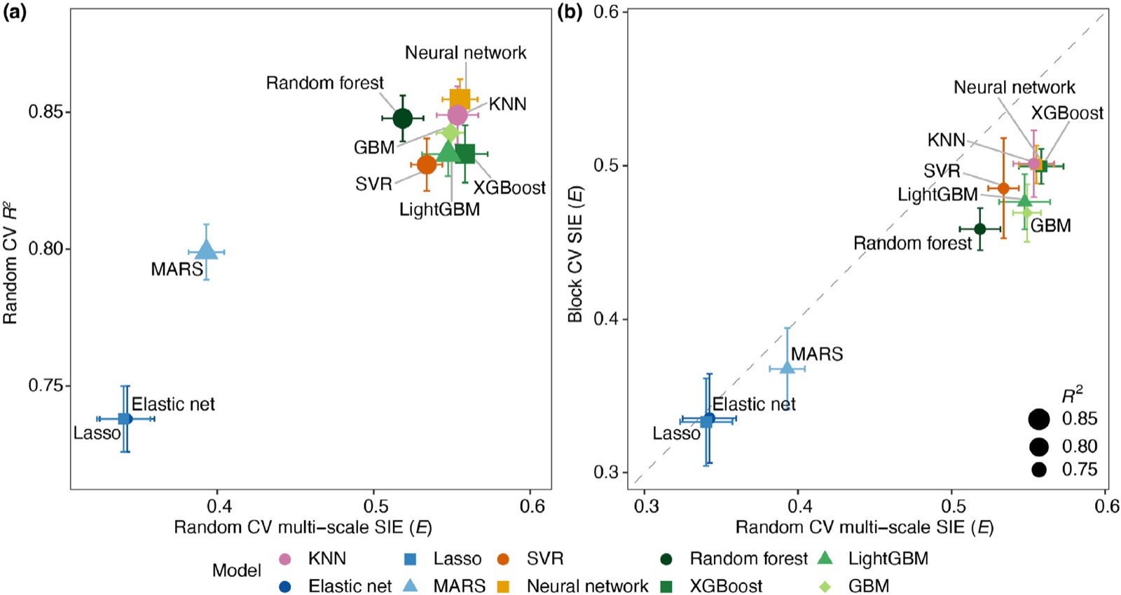
KNN, the neural network and XGBoost formed a statistically indistinguishable leading group with E of about 0.50, and the ranking was robust to five alternative random assignments of blocks to folds. Support vector regression had the lowest RMSE (8.26) and highest R2 (0.789), and random forest the second-lowest RMSE but the seventh-highest E, which the paper relates to the smoothing of its averaged response surface. Across the ten models the Spearman rank correlation of E was −0.38 with RMSE and 0.53 with R2, and the paper concludes that prediction accuracy and explained spatial information are distinct, complementary dimensions of model quality. The neural network and support vector regression gave the strongest combination of both (Figure 6).[1] Residual maps of the higher-SIE models showed weaker large-scale gradients in central and southern Australia, while all models retained residual clustering in the tropical north and semi-arid interior.
Sensitivity to discretization
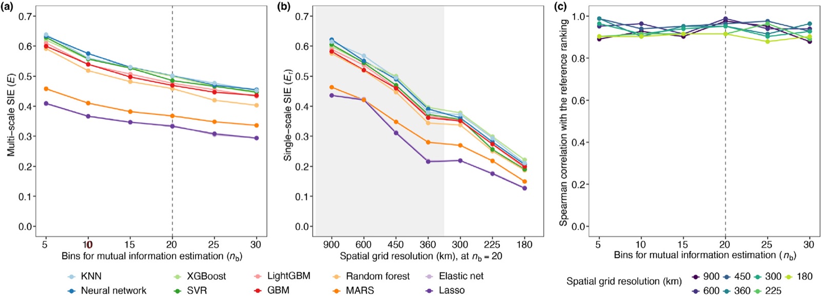
Recomputing E from the same block cross-validation residuals for 42 combinations of bin count (5 to 30) and grid resolution (900 to 180 km) showed that discretization affects the magnitude of E but hardly the ranking of models (Figure 8). Mean single-scale Er fell from 0.552 at 900 km to 0.181 at 180 km as the bias term rose from 0.05 to 0.95 nats while I(Y; S) rose only from 0.67 to 1.58. The Spearman correlation between each setting's ranking and the reference ranking was at least 0.879 (median 0.927); the top rank stayed within the leading group in 40 of the 42 settings, and the regularized linear models ranked lowest in all of them. The paper accordingly recommends choosing settings so that the leading bias term is small relative to I(Y; S) — at most about 0.25 of it in the case study.[1]
Block versus random cross-validation
Under random cross-validation, RMSE was lower (mean 8.15 against 9.12) and R2 higher (0.815 against 0.734) than under block cross-validation, and E was higher for all ten models (mean 0.489 against 0.443). The overstatement of E ranged from 2.1% for the regularized linear models to 17.0% for gradient boosting, with a mean of 9.9%, and was largest for high-capacity models able to exploit spatial proximity (Figure 9). The paper attributes the inflation of both accuracy and SIE to the same mechanism: under random partitioning, nearby training observations reproduce local spatial structure that the predictors alone cannot supply, so block cross-validation gives the more conservative estimate of spatial learning when the aim is generalization to unobserved regions.[1]
Relationship to other methods
The paper positions SIE among evaluation methods for spatial prediction by evaluation objective and spatial analytical capacity (Table 4). Accuracy metrics such as RMSE and R2 quantify error magnitude. SHAP and GeoShapley attribute predictions to predictors and to location without quantifying explained spatial information.[14] Among residual-based methods from the same research group, the generalized spatial error evaluates local prediction errors,[7] the degree of spatial interpretability (DSI) quantifies the spatially stratified variance a model explains,[5] and the degree of geocomplexity (DG) the loss of local spatial pattern.[6] SIE differs in measuring the relative reduction of spatial information through mutual information, which captures general statistical dependence on location, and in integrating it across scales from spatially separated validation predictions.
| Capability | RMSE / R2 | SHAP | GeoShapley | GSE | DSI | DG | SIE |
|---|---|---|---|---|---|---|---|
| Prediction error magnitude | ✓ | × | × | ✓ | × | × | × |
| Predictor variable attribution | × | ✓ | ✓ | × | × | × | × |
| Geographic location attribution | × | × | ✓ | × | × | × | × |
| Spatial information explained | × | × | × | × | ✓ | ✓ | ✓ |
| Local errors explained | × | × | × | ✓ | × | × | × |
| Spatial dependence assessed | × | × | × | × | ✓ | × | ✓ |
| Spatial heterogeneity captured | × | × | × | × | ✓ | × | ✓ |
| Geocomplexity captured | × | × | × | × | × | ✓ | ✓ |
| General statistical spatial characteristics | × | × | × | × | × | × | ✓ |
| Residual spatial structure assessed | × | × | × | ✓ | ✓ | ✓ | ✓ |
| Multi-scale spatial assessment | × | × | × | × | × | × | ✓ |
Source: Song (2026), Table 4. ✓ indicates that the capability is present, × that it is absent. GSE = generalized spatial error; DSI = degree of spatial interpretability; DG = degree of geocomplexity.
Moran's I of residuals tests whether neighbouring residuals are more similar than expected under spatial randomness, and Moran eigenvector spatial filtering has been used to reduce such autocorrelation in machine learning models;[17] it detects unexplained dependence but does not quantify what share of the response's spatial information remains. The area of applicability identifies the predictor space within which predictions can be considered reliable,[15] and is complementary. Spatial+ cross-validation is complementary in the design dimension: SIE can be computed from the residuals of any spatially separated validation design, including spatial+ partitions.[16] A summary of the related methods from the research group is maintained on the Methods page.
The paper names three directions for further work: continuous estimators of mutual information, such as kernel and k-nearest-neighbour estimators, and continuous-scale SIE over the bounded resolution range; the integration of SIE into automated model selection and spatial deep learning; and evaluation with responses of different spatial dependence, categorical responses such as land cover, and other geographic domains.[1]
Software
SIE is implemented in a single base-R file released with the paper. The function takes observed values, out-of-fold predictions and coordinates, so it can be applied to the output of any model and any spatially separated validation design.
GitHub repository
The sie() function, the C4 grass data for 2,480 grid cells, and an example that rebuilds the ten-model comparison and checks it against reference results.
Reproducing SIE
One-command pipeline that re-runs the case study, works through a hand-checkable example, and redraws the case-study figures.
yongzesong.com/reproduce/sie.htmlMinimal example
source("sie.R")                      # from github.com/yongzesong/SIE, base R only
c4 <- read.csv("c4-data.csv")         # 2,480 cells: lon, lat, response, 3 predictors

# y_hat: out-of-fold predictions of a model from spatial block cross-validation
# (example.R builds them for the ten models of the paper)
E <- sie(y = c4$C4_grass_area_pct, y_hat = y_hat,
         coords = c4[, c("lon", "lat")], n_bins = 20, scales = c(4, 6, 8, 10))
E$E          # multi-scale SIE, e.g. 0.501 for k-nearest neighbours
E$profile    # per grid: occupied cells, I(Y;S), I(e;S), E_r, bias term, weight
Call sequence from the repository README; scales gives the grid sizes g of g × g cells over the bounding box of the coordinates.
References
- Song, Y. (2026). Spatial information explained by prediction models under block cross-validation. ISPRS Journal of Photogrammetry and Remote Sensing, 242, 984–1000. doi:10.1016/j.isprsjprs.2026.09.034
- Ploton, P., et al. (2020). Spatial validation reveals poor predictive performance of large-scale ecological mapping models. Nature Communications, 11, 4540.
- De Bruin, S., Brus, D.J., Heuvelink, G.B.M., van Ebbenhorst Tengbergen, T., & Wadoux, A.M.J.-C. (2022). Dealing with clustered samples for assessing map accuracy by cross-validation. Ecological Informatics, 69, 101665.
- Bates, S., Hastie, T., & Tibshirani, R. (2024). Cross-validation: what does it estimate and how well does it do it? Journal of the American Statistical Association, 119, 1434–1445.
- Liu, H., Song, Y., & Yi, W. (2026). Degree of spatial interpretability. International Journal of Geographical Information Science. doi:10.1080/13658816.2026.2614335
- Liu, H., Song, Y., Yi, W., & Zhang, P. (2026). Degree of geocomplexity for diagnosing spatial pattern loss beyond prediction accuracy. GIScience & Remote Sensing, 63(1), 2657087.
- Liu, H., Song, Y., Zhang, P., Ren, K., & Wu, Y. (2026). Generalised spatial error for validation. GIScience & Remote Sensing, 63(1), 2690327.
- Zhang, Z., Song, Y., Luo, P., & Wu, P. (2023). Geocomplexity explains spatial errors. International Journal of Geographical Information Science, 37(7), 1449–1469.
- Zhang, W.B., Ge, Y., Bai, H., Jin, Y., Stein, A., & Atkinson, P.M. (2023). Spatial association from the perspective of mutual information. Annals of the American Association of Geographers, 113, 1960–1976.
- Miller, G.A. (1955). Note on the bias of information estimates. In H. Quastler (Ed.), Information Theory in Psychology: Problems and Methods (pp. 95–100). Free Press.
- Paninski, L. (2003). Estimation of entropy and mutual information. Neural Computation, 15, 1191–1253.
- Luo, X., et al. (2024). Mapping the global distribution of C4 vegetation using observations and optimality theory. Nature Communications, 15, 1219.
- Song, I., & Kim, D. (2023). Three common machine learning algorithms neither enhance prediction accuracy nor reduce spatial autocorrelation in residuals: an analysis of twenty-five socioeconomic data sets. Geographical Analysis, 55, 585–620.
- Li, Z. (2024). GeoShapley: a game theory approach to measuring spatial effects in machine learning models. Annals of the American Association of Geographers, 114, 1365–1385.
- Meyer, H., & Pebesma, E. (2021). Predicting into unknown space? Estimating the area of applicability of spatial prediction models. Methods in Ecology and Evolution, 12(9), 1620–1633.
- Wang, Y., Khodadadzadeh, M., & Zurita-Milla, R. (2023). Spatial+: a new cross-validation method to evaluate geospatial machine learning models. International Journal of Applied Earth Observation and Geoinformation, 121, 103364.
- Islam, M.D., Li, B., Lee, C., & Wang, X. (2022). Incorporating spatial information in machine learning: the Moran eigenvector spatial filter approach. Transactions in GIS, 26, 902–922.
Citing SIE
@article{song2026sie,
  title   = {Spatial information explained by prediction models under block
             cross-validation},
  author  = {Song, Yongze},
  journal = {ISPRS Journal of Photogrammetry and Remote Sensing},
  volume  = {242},
  pages   = {984--1000},
  year    = {2026},
  doi     = {10.1016/j.isprsjprs.2026.09.034}
}
External links
- Full text of the paper at ScienceDirect (open access)
- SIE on GitHub
- Reproducing SIE (tutorial)
- Spatial validation methods of the research group