Generalized covariate field
Song, Y. (2026). Generalized covariate field (GCF): spatial-pattern and neighbourhood-distribution feature expansion improves geospatial prediction. International Journal of Geographical Information Science, 40, 1–29. https://doi.org/10.1080/13658816.2026.2729719
Full text · BibTeX · R package · Code · Web appThe generalized covariate field (GCF) is a spatial representation model for geospatial prediction that expands each explanatory variable, or covariate, from its value at a location into a set of features describing the spatial structure and neighbourhood distribution of that covariate around the location.[1] The model was introduced by Yongze Song in 2026 in the International Journal of Geographical Information Science. GCF is intended for prediction problems in Earth and environmental sciences in which the response variable is observed at sparse or unevenly distributed sample locations, while covariates are available continuously across the study area, including at locations where no response has been observed.
GCF organizes predictors into three categories: the original predictors, spatial pattern features derived by applying eleven neighbourhood operators to each covariate, and neighbourhood distribution features obtained by summarizing covariate values within multiscale neighbourhoods using quantiles. The resulting high-dimensional candidate set is reduced by a two-stage variable selection procedure consisting of response-independent functional reduction and spatial-block stability selection, after which any supervised learner may be trained on the selected features.[1] The term generalized refers to the fact that three conventional predictor sets, namely covariates alone, covariates with spatial features, and covariates with neighbourhood statistics, arise as special cases of the GCF representation.
In a case study predicting vascular plant species richness across the Southwest Australian Floristic Region, GCF expanded 12 environmental covariates into 3,276 candidate predictors and improved spatial-block cross-validated R2 by 8.2–21.1% relative to covariate-only models across seven learners.[1] The results are presented as support for the primacy of data hypothesis, which holds that enriching the spatial representation of data can improve prediction more than increasing model structural complexity.
Background
Spatial prediction supports tasks such as climate modelling, biodiversity monitoring, ecosystem assessment, and natural hazard forecasting, and requires reliable estimates at unsampled or sparsely monitored locations as well as at observed ones.[2] Although advances in remote sensing have increased the availability and resolution of spatial data, more data alone does not guarantee higher prediction accuracy for complex systems,[3] and prediction remains constrained by spatial heterogeneity and by sparse, uneven sampling.
Methods for spatial prediction are commonly grouped into spatial statistical models such as kriging, spatial autoregressive models and geographically weighted regression; spatially informed machine learning, including random forests, gradient boosting and support vector machines with spatial covariates; and hybrid approaches, including deep learning architectures such as graph convolutional networks.[1] A recurring observation in this literature is that many machine learning models treat observations as independent and do not represent spatial structure, and that emerging approaches address this either by embedding spatial variables into the input space or by adapting the learning algorithm.
GCF belongs to the first of these strategies. Its starting point is the covariate field: because covariates are typically observed on a support that extends beyond the response sample locations, their local distributions and spatial patterns around each prediction location carry information that point covariate values do not.[4] Earlier work by the same research group on the second dimension of spatial association,[5] geocomplexity,[6] and second-dimension outliers[7] examined individual aspects of this information. GCF was developed to generate and integrate spatial pattern and neighbourhood distribution features from covariates systematically, at both sampled and unsampled locations, within a single construction.
Definition
Let 𝒟 denote the study domain, 𝒮 ⊂ 𝒟 the sampled locations u at which both covariates x(u) and the response y(u) are observed, and 𝒢 ⊂ 𝒟 the prediction grid of locations v at which covariates are available but the response is unobserved. GCF predicts the response at a sampled location through
where the GCF feature vector
is defined at every location s with covariate support, and the learner f is any supervised model. The methodological contribution of GCF lies in the construction of Φ rather than in the choice of f.[1]
The paper defines the spatial representation of data as the quantities supplied to a learner as predictors for each location, comprising the covariate values at that location together with quantities encoding the spatial structure of the covariate field in its neighbourhood. Under this definition, the covariate vector x(s) is the point-support representation and Φ(s) is an enriched representation built from the same observations without adding response samples.
Predictor categories
GCF organizes predictors into three categories, each retaining the identity of the covariate from which it is derived:
- Original predictors x: the covariate values at the location itself, as used by conventional models.
- Spatial pattern features ψ(x): descriptors of local spatial structure produced by a spatial pattern operator acting on the covariate field within a neighbourhood 𝒩(s). They characterize spatial dependence, local heterogeneity, distributional diversity, geocomplexity, multiscale variation and local outlyingness, and are designed to be transferable across space.
- Neighbourhood distribution features Zx: distributional summaries of covariate values within multiscale neighbourhoods 𝒩(s; b) of buffer radius b, indexed by quantile level τ.
The construction is implemented in four steps: generation of spatial pattern features, generation of neighbourhood distribution features, variable selection, and spatial learning.
Spatial pattern features
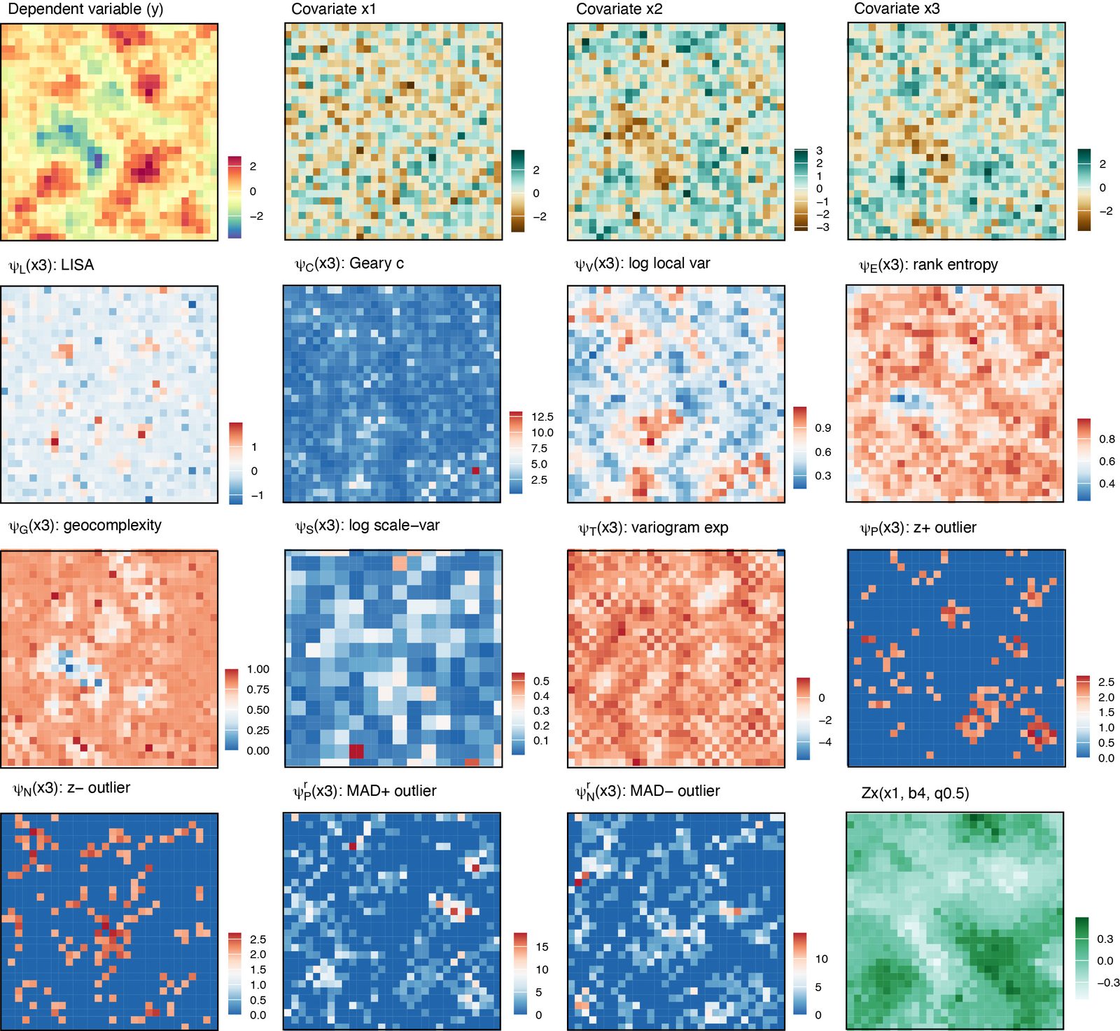
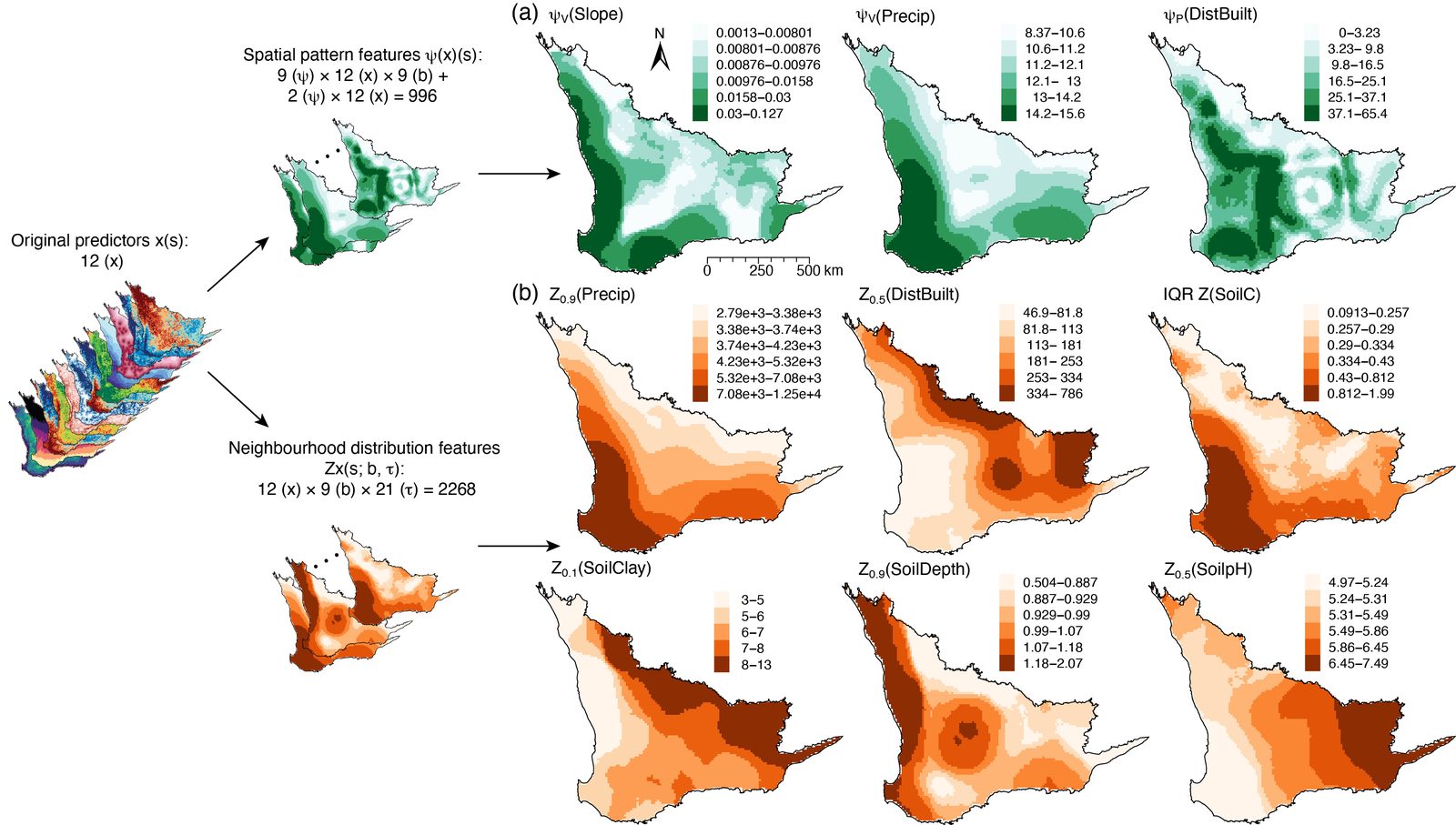
For each covariate x, the spatial pattern operator produces an h-dimensional vector ψ(x)(s) = (ψ1(x)(s), …, ψh(x)(s)), where each component is computed from the values of x within the neighbourhood 𝒩(s). The same set of operators is applied independently to every covariate. The published implementation uses eleven operators in six categories.[1]
| Category | Operator | Symbol | What it measures | Origin |
|---|---|---|---|---|
| Spatial dependence | Transferable LISA-type statistic | ψL | Local spatial association computed from locally standardized values, removing broad-scale differences in level and variability | Adapted from local indicators of spatial association[8] |
| Local Geary's c | ψC | Mean squared difference between a location and its neighbours | Anselin (1995)[8] | |
| Local heterogeneity | Log local variance | ψV | Variability of covariate values within the neighbourhood | Woodcock & Strahler (1987) |
| Distributional diversity | Rank-binned entropy | ψE | Evenness of neighbourhood values across global rank bins | Batty (1974) |
| Geocomplexity | Geocomplexity | ψG | Local spatial complexity accounting for neighbour dependence | Zhang et al. (2023)[6] |
| Multiscale variation | Log scale-variance index | ψS | Variance of block means across nested grid scales | Moellering & Tobler (1972) |
| Local variogram exponent | ψT | Log-log slope of the local semivariogram | Oliver & Webster (2014) | |
| Local outlyingness | Local-z positive outlier strength | ψP | Summed magnitude of neighbours exceeding a positive z-score threshold | Ren et al. (2026)[7] |
| Local-z negative outlier strength | ψN | Summed magnitude of neighbours below a negative z-score threshold | Ren et al. (2026)[7] | |
| Robust positive outlier strength | ψPr | As ψP, using the local median and median absolute deviation | Aggarwal (2017) | |
| Robust negative outlier strength | ψNr | As ψN, using the local median and median absolute deviation | Aggarwal (2017) |
Nine of the eleven operators depend on the neighbourhood radius and are evaluated at each buffer radius, while two are scale-invariant and are computed once per covariate. The operator set is open: any functional of covariate values over a defined spatial support can be added without altering the construction.
Neighbourhood distribution features
Neighbourhood distribution features summarize the distribution of covariate values surrounding each location. For a covariate x, a set of buffer radii b ∈ ℬ defines multiscale neighbourhoods, and within each neighbourhood a distribution-summary operator Qτ, taken as the quantile at level τ, is applied to the covariate values at locations with covariate support:[5]
Each buffer–quantile combination yields one feature. Covariates are kept at their native resolution, so the construction does not require all covariates to be resampled to a common grid. Although quantiles are used in the published implementation, Qτ may be replaced by other distributional summaries such as means, upper-tail statistics, threshold exceedances or entropy.
Variable selection
The candidate set formed by the three predictor categories is high-dimensional and strongly collinear, because neighbouring buffers, adjacent quantile levels and related operators encode similar information. GCF applies a two-stage selection procedure.[1]
Response-independent functional reduction. The buffer set is partitioned into a fine band and a broad band, preserving a near–far contrast. Within each band, the neighbourhood distribution features of a covariate are collapsed into five functionals of the quantile curve: the median, the interquartile range, the lower tail, the upper tail and a skew descriptor. Scale-dependent spatial pattern operators are averaged within each band, and scale-invariant operators pass through unchanged. Because this stage uses covariate information only, it introduces no response leakage.
Spatial-block stability selection. The original predictors are forced into all models and are exempt from selection, so that derived features compete only for information beyond that already represented by x. The study region is partitioned into contiguous square blocks. In each of M resampling rounds, a fraction γ of blocks is sampled, a random forest is fitted, and the top k derived features by impurity importance are marked as selected. Features are grouped by covariate and feature category, and the selection frequency of a group g is
where δrj = 1 if feature j is selected in round r. Groups with p̂g ≥ π are retained, and each retained group contributes one representative feature, the member with the highest mean selection frequency. The final predictor set is the union of the forced original predictors and the representative derived features. In cross-validation, the whole procedure is re-estimated within each training fold.
Spatial learning and prediction
A supervised learner is trained on the selected feature vector Φ𝒜(u) evaluated at the sampled locations, and prediction at an unknown location v ∈ 𝒢 is given by ŷ(v) = f(Φ𝒜(v)). Because the features are computed wherever covariates are available, the same construction serves both training and prediction, and the predictions form a surface over the prediction grid. The published study uses random forest as the adopted learner and reports six comparison learners.
Conditions for benefit
The paper states three conditions that govern when GCF is expected to improve prediction:[1]
- The response depends on the geographical context of a location rather than on its point covariate values alone.
- Covariates are observed on a support extending beyond the response sample locations, so that neighbourhood summaries carry information the response samples do not.
- The neighbourhood radii span the scales at which the underlying process operates.
Under these conditions, the expected gain increases as the response sample becomes sparser relative to the covariate support, because neighbourhood features supply contextual information unavailable at the sampled locations. Improvements are correspondingly smaller where response sample density approaches the covariate resolution, so that neighbourhood summaries duplicate information already in x, or where the process scale falls outside the range spanned by the buffer radii. The paper also notes that the implemented operators describe local heterogeneity, and that populations dominated by stratified heterogeneity would call for stratum-based operators within the same construction.[9]
Evaluation
GCF was evaluated in a controlled simulation and in an application to plant species richness. Both used five-fold random cross-validation and five-fold spatial-block cross-validation, with variable selection re-estimated in each training fold, and compared GCF models with covariate-only models across seven learners: linear regression (LM), GLMNET, random forest (RF), Cubist, distance-weighted k-nearest neighbours (KNN), XGBoost and a radial-kernel support vector machine (SVM).[1]
Simulation study
The simulation used a regular 30 × 30 grid with a response generated as a spatially autocorrelated Gaussian random field and three explanatory variables formed by adding spatially independent noise to that field (Figure 1). With buffer radii {2, 4, 6}, a normalization radius of 4 and quantile levels from 0 to 1 in steps of 0.1, each explanatory variable produced 63 predictors (1 original, 29 spatial pattern and 33 neighbourhood distribution features), giving 189 candidates in total.
| Learner | R2, covariate-only | R2, GCF | Improvement | RMSE, covariate-only | RMSE, GCF | Improvement |
|---|---|---|---|---|---|---|
| LM | 0.469 | 0.668 | +42.4% | 0.706 | 0.551 | +22.0% |
| GLMNET | 0.470 | 0.668 | +42.1% | 0.707 | 0.552 | +22.0% |
| RF | 0.419 | 0.657 | +56.5% | 0.741 | 0.561 | +24.3% |
| Cubist | 0.438 | 0.637 | +45.6% | 0.728 | 0.575 | +21.0% |
| KNN | 0.429 | 0.637 | +48.5% | 0.736 | 0.578 | +21.5% |
| XGBoost | 0.399 | 0.619 | +55.2% | 0.754 | 0.590 | +21.8% |
| SVM | 0.433 | 0.591 | +36.6% | 0.734 | 0.624 | +15.0% |
Source: Song (2026), Table 2. Improvement is the relative change from the covariate-only model to the GCF model. Random cross-validation results follow the same pattern.
Under spatial-block cross-validation, GCF models achieved R2 between 0.591 (SVM) and 0.668 (LM), compared with 0.399–0.470 for covariate-only models. All seven learners improved under both cross-validation schemes, which the paper interprets as evidence that the improvement is attributable to the GCF representation rather than to any particular learning algorithm. The strong performance of the GCF-based linear model is attributed to the spatial pattern and neighbourhood distribution features encoding much of the spatial structure before model fitting, leaving a comparatively simple mapping from predictors to response.
Case study: plant species richness in southwestern Australia
The application predicted vascular plant species richness across the Southwest Australian Floristic Region (SWAFR), a global biodiversity hotspot with approximately 7,380 native vascular plant species and subspecies, about half of them endemic.[10] Richness observations from 4,989 plots of 400 m2[11] were aggregated to a 10 km grid, yielding 958 spatial units with values ranging from 0.4 to 135.8 (mean 41.1). Twelve covariates in three groups were used: geography (elevation, slope), climate and environment (total precipitation over 2013–2023, shortwave radiation, distance to water, distance to built-up areas), and soil properties (nitrogen, organic carbon, clay fraction, depth, pH, bulk density).
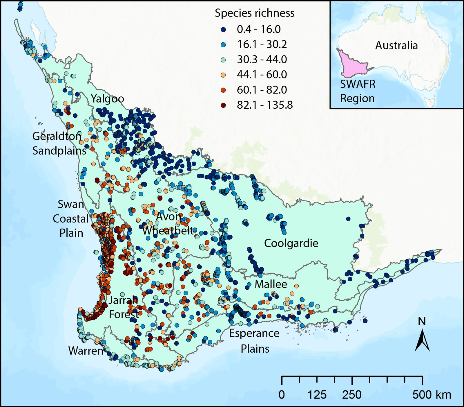
Spatial pattern features were computed over buffer radii of 20 to 100 km in 10 km steps, with a normalization radius of 100 km, and neighbourhood distribution features over the same nine radii at 21 quantile levels. The 12 covariates were thereby expanded into 12 original predictors, 996 spatial pattern features and 2,268 neighbourhood distribution features, a total of 3,276 candidates. Functional reduction with a fine band of {20, 30} km and a broad band of {90, 100} km reduced the set to 372 features. Stability selection used 80 rounds, a block sampling fraction of 0.7, 200-tree random forests, the top 20 features per round, and a retention threshold of 0.6. Applied to the full sample, the procedure retained 9 of 24 covariate-by-category groups, so the final model comprised the 12 original covariates and 9 representative derived features, all located in the 90–100 km broad scale band (Figure 3).
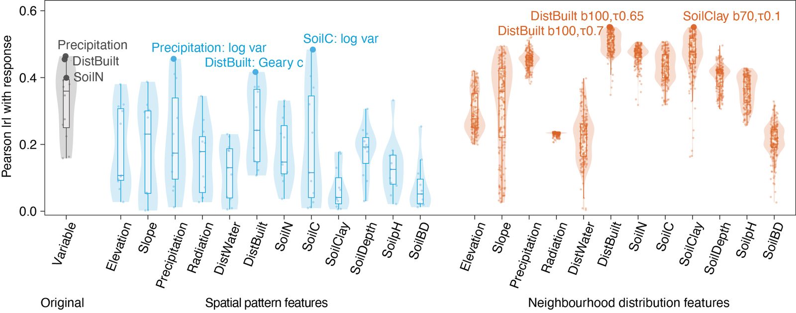
Spatial-block cross-validation used square blocks of side 132 km, twice the spatial-dependence range of about 66 km estimated from the residual variogram of species richness after removing the covariate trend, giving 38 occupied blocks assigned to five spatially disjoint folds.
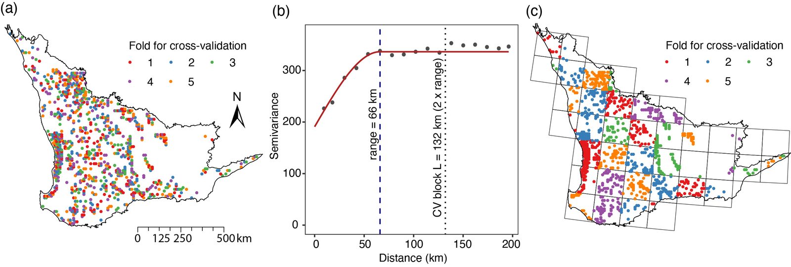
| Learner | R2, covariate-only | R2, GCF | Improvement | RMSE, covariate-only | RMSE, GCF | Improvement |
|---|---|---|---|---|---|---|
| RF (adopted) | 0.296 | 0.346 | +16.7% | 17.966 | 17.428 | +3.0% |
| Cubist | 0.283 | 0.342 | +21.1% | 18.065 | 17.506 | +3.1% |
| KNN | 0.296 | 0.320 | +8.2% | 18.039 | 17.743 | +1.6% |
| XGBoost | 0.261 | 0.315 | +20.3% | 18.304 | 17.795 | +2.8% |
| SVM | 0.275 | 0.327 | +18.6% | 18.489 | 17.849 | +3.5% |
| GLMNET | 0.259 | 0.302 | +16.9% | 18.575 | 18.054 | +2.8% |
| LM | 0.253 | 0.286 | +13.0% | 18.647 | 18.279 | +2.0% |
Source: Song (2026), Table 5. Under random cross-validation the corresponding R2 improvements were 0.7–13.2%.
Every learner improved under GCF in both schemes. Under spatial-block cross-validation, R2 increased by 8.2–21.1% and RMSE fell by 1.6–3.5%; under random cross-validation the gains were smaller, at 0.7–13.2% in R2. The larger gains under the stricter spatial-block scheme are interpreted as improved transferability to spatially separated and unsampled areas. A feature-set comparison with random forest showed that adding spatial pattern features alone raised spatial-block R2 from 0.296 to 0.337, adding neighbourhood distribution features alone raised it to 0.329, and the full GCF representation reached 0.346. A Shapley decomposition of the GCF R2 attributed 45.6% to the original covariates, 24.8% to spatial pattern features and 29.6% to neighbourhood distribution features.
Robustness
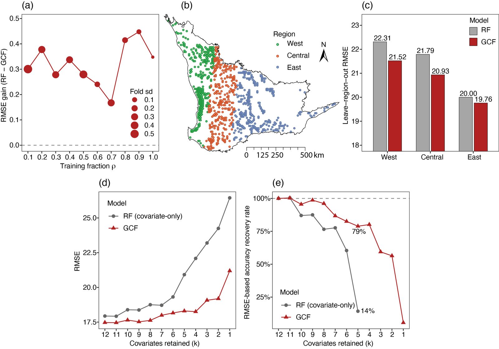
Three experiments examined the robustness of the GCF gain (Figure 6). Under sparse sampling, the RMSE gain relative to covariate-only random forest remained positive at all training fractions, increasing from 0.30 at a training fraction of 0.1 to 0.45 at 0.9. In leave-region-out validation, GCF reduced RMSE in all three withheld regions, by 0.85 in the central, 0.79 in the western and 0.24 in the eastern region. Under covariate scarcity, with the strongest covariates removed first, GCF recovered 79% of the full-covariate prediction capacity with five covariates retained, compared with 14% for covariate-only random forest; with a single covariate, RMSE rose by 21% for GCF and 47% for the covariate-only model, and GCF maintained positive R2 throughout whereas the covariate-only model did not when fewer than four covariates remained.
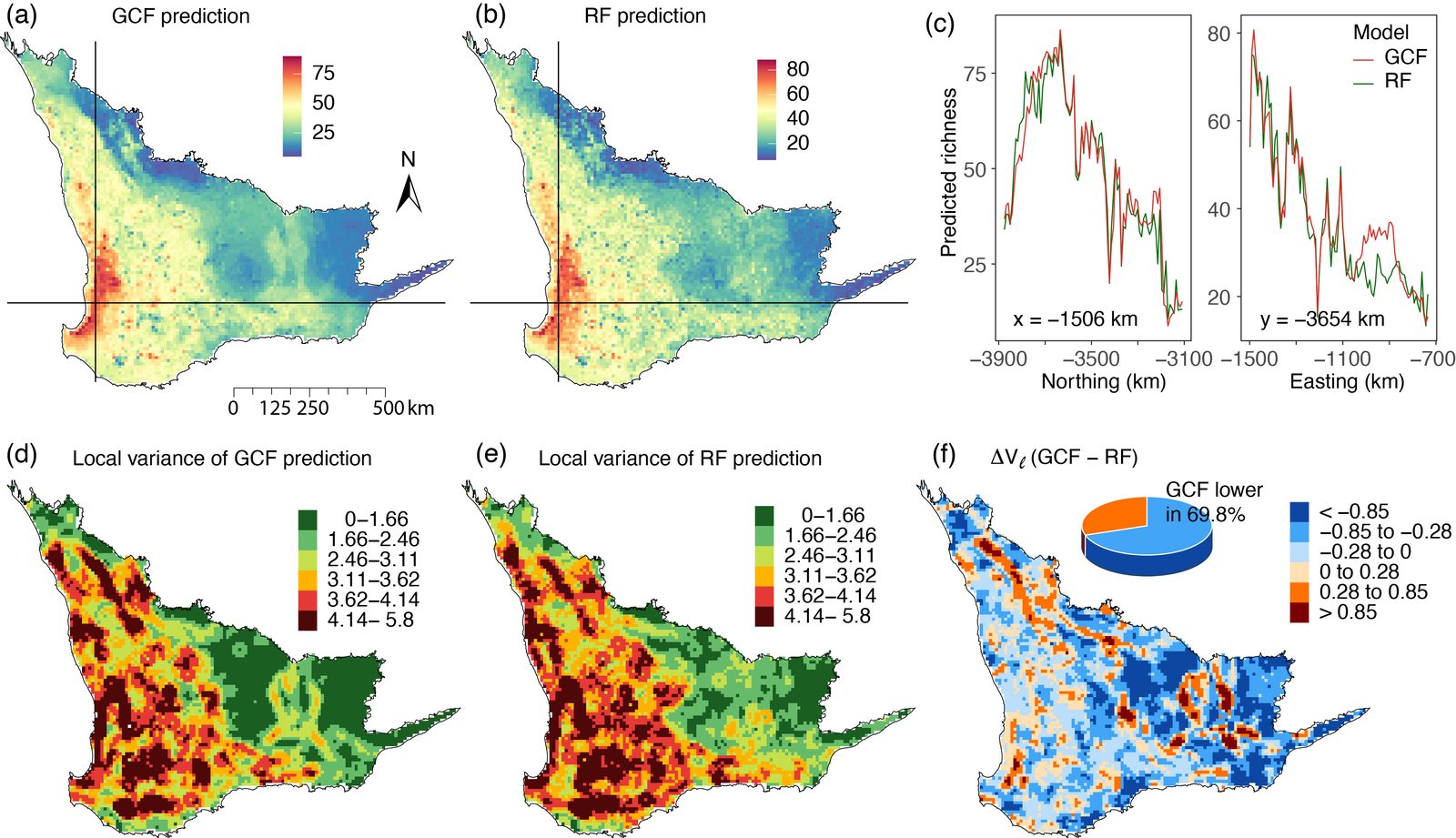
When refitted on all samples and mapped across the prediction grid, the GCF surface showed smoother spatial transitions than the covariate-only random forest surface while preserving high- and low-richness contrasts along cross-sections, and had lower local variance across 69.8% of the region (Figure 7).
Primacy of data
The paper frames its results as support for what it calls the primacy of data hypothesis: that enriching the spatial representation of data, rather than only increasing model structural complexity, can substantially improve prediction.[1] The clearest illustration is the simulation, in which a linear model fitted to GCF features reached a spatial-block R2 of 0.668, above the covariate-only random forest (0.419) and XGBoost (0.399). The argument is that spatial structure that a flexible learner would otherwise need to discover from sparse response data is instead computed explicitly from the covariate field, where it is observable everywhere, and supplied as predictors. This positions GCF within data-centric approaches to geospatial modelling, in which effort is directed to the representation supplied to a model rather than to the model architecture.
Relationship to other methods
Special cases. Three predictor sets used in existing spatial prediction are nested within GCF: the covariates alone (x), covariates with spatial features (x + ψ), and covariates with neighbourhood statistics (x + Zx). In the biodiversity case each of these sets performed below the full representation, and the paper presents this as the sense in which the covariate field is generalized.
Kriging, spatial regression and geographically weighted regression model spatial dependence or spatially varying coefficients in the response, using covariate values at the point of prediction. GCF is complementary: it changes the predictor set, not the learner, and its features may be supplied to such models as covariates.
Focal statistics and neighbourhood summaries in GIS and remote sensing compute moving-window statistics of a raster. The neighbourhood distribution operator of GCF is of this family, extended to multiscale radii and full quantile curves, and combined with a selection procedure designed to prevent response leakage and to enforce spatial reproducibility.
Related methods from the same research group include the second dimension of spatial association,[5] which relates a location to the distribution of values in its neighbourhood and underlies the neighbourhood distribution operator; geocomplexity,[6] which is one of the spatial pattern operators; second-dimension outliers for spatial prediction,[7] on which the outlier-strength operators draw; geographically optimal similarity,[12] which predicts from structurally similar observations rather than proximity; the generalized heterogeneity model,[13] which addresses stratified heterogeneity in interpolation; and focal-feature regression kriging.[4] A summary of these methods is maintained on the Methods page.
Software
GCF is implemented in open-source software released with the paper. The feature construction and variable selection are provided independently of any learner, so that users may pair the representation with their preferred model.
gcf on CRAN
Generates GCF variables from spatial covariates and selects a stable subset for any downstream regression learner. Install with install.packages("gcf").
GCF Calculator
Runs in the browser without installation. Upload a CSV of coordinates and covariates to generate GCF features and run stability selection.
yongzesong.com/app/gcf/GitHub repository
Single-file R implementation with the same function names as the package, an example script and simulated data.
github.com/yongzesong/gcfReproducing GCF
One-command pipeline that re-runs the simulation and rebuilds the published tables and prediction figure.
yongzesong.com/reproduce/gcf.htmlMinimal example
install.packages("gcf")   # from CRAN
library(gcf)
data(sim_grid)   # 30 x 30 grid, 900 rows: y1, x1, x2, x3, x, y

# Steps 1-3a: spatial pattern and neighbourhood distribution features,
# then response-independent functional reduction (paper's simulation settings)
field  <- gcf_field(sim_grid, coords = c("x", "y"), vars = c("x1", "x2", "x3"),
                    buffers = c(2, 4, 6), probs = seq(0, 1, 0.1),
                    d_norm = 4, fine_band = 2, broad_band = 6)

# Step 3b: spatial blocks and stability selection (raw covariates are forced in)
blocks <- gcf_blocks(sim_grid[, c("x", "y")], size = 6)
sel    <- gcf_select(field, y = sim_grid$y1, blocks = blocks)   # B = 80, pi_thr = 0.6

# Step 4: any learner on the selected predictors
train  <- cbind(y1 = sim_grid$y1, field$candidates[, sel$selected])
fit    <- lm(y1 ~ ., data = train)
Call sequence from the package examples; field$candidates holds the reduced candidate set and sel$selected the forced covariates followed by the group representatives.
References
- Song, Y. (2026). Generalized covariate field (GCF): spatial-pattern and neighbourhood-distribution feature expansion improves geospatial prediction. International Journal of Geographical Information Science, 40, 1–29. doi:10.1080/13658816.2026.2729719
- Meyer, H., & Pebesma, E. (2021). Predicting into unknown space? Estimating the area of applicability of spatial prediction models. Methods in Ecology and Evolution, 12(9), 1620–1633.
- Chi, M., et al. (2016). Big data for remote sensing: Challenges and opportunities. Proceedings of the IEEE, 104(11), 2207–2219.
- Luo, P., Wu, Y., & Song, Y. (2026). Focal-feature regression kriging. Geographical Analysis, 58(2), e70035.
- Song, Y. (2022). The second dimension of spatial association. International Journal of Applied Earth Observation and Geoinformation, 111, 102834.
- Zhang, Z., et al. (2023). Geocomplexity explains spatial errors. International Journal of Geographical Information Science, 37(7), 1449–1469.
- Ren, K., Song, Y., & Yu, Q. (2026). Second-dimension outliers for spatial prediction. International Journal of Geographical Information Science, 40(6), 1915–1942.
- Anselin, L. (1995). Local indicators of spatial association—LISA. Geographical Analysis, 27(2), 93–115.
- Wang, J.F., et al. (2010). Geographical detectors-based health risk assessment and its application in the neural tube defects study of the Heshun region, China. International Journal of Geographical Information Science, 24(1), 107–127.
- Hopper, S.D., & Gioia, P. (2004). The Southwest Australian Floristic Region: evolution and conservation of a global hot spot of biodiversity. Annual Review of Ecology, Evolution, and Systematics, 35, 623–650.
- Mokany, K., et al. (2022). Patterns and drivers of plant diversity across Australia. Ecography, 2022(11), e06426.
- Song, Y. (2023). Geographically optimal similarity. Mathematical Geosciences, 55(3), 295–320.
- Luo, P., et al. (2023). A generalized heterogeneity model for spatial interpolation. International Journal of Geographical Information Science, 37(3), 634–659.
Citing GCF
@article{song2026gcf,
  title   = {Generalized covariate field ({GCF}): spatial-pattern and neighbourhood-distribution
             feature expansion improves geospatial prediction},
  author  = {Song, Yongze},
  journal = {International Journal of Geographical Information Science},
  volume  = {40},
  pages   = {1--29},
  year    = {2026},
  doi     = {10.1080/13658816.2026.2729719}
}

@Manual{song2026gcfpkg,
  title   = {gcf: Generalized Covariate Field},
  author  = {Song, Yongze},
  year    = {2026},
  note    = {R package version 0.1.0},
  doi     = {10.32614/CRAN.package.gcf},
  url     = {https://CRAN.R-project.org/package=gcf}
}
External links
- Full text of the paper at Taylor & Francis Online
- gcf R package on CRAN
- gcf on GitHub
- Data and codes on Figshare
- GCF Calculator (browser application)
- Reproducing GCF (tutorial)