Reproducing the Spatial Trade-Off Relation (STOR) Model
A complete walkthrough of the STOR model — which measures the
quantity and quality of infrastructure as two entropy-weighted indices, reads their
relation as a utility function, and cuts it into stages of diminishing marginal utility — from
block-level indicators to manuscript. The method is implemented here in a single self-contained
R file with no package dependency, demonstrated end to end on simulated data with a known
trade-off hidden inside.
R/ pipeline scripts including the complete method in
R/02-stor-core.R · config/project-config.R · data/
(1,600 simulated blocks with 14 indicators and the embedded ground truth) · tests/ ·
run-all.R — unzip and run Rscript run-all.R test from the
STOR/ folder root.
To cite the STOR model in publications, please use:
Song Y, Wu P, Hampson K, Anumba C (2021). Assessing block-level
sustainable transport infrastructure development using a spatial trade-off relation model.
Int J Appl Earth Obs Geoinf 105:102585.
doi ·
PDFCC BY-NC-ND
1 Method Overview & Reproduction Scope
1.1 Core Idea
Building more roads and building better roads are both pathways to sustainable
infrastructure, and they compete for the same budget. Song et al. (2021) make that
competition measurable. Every spatial unit — 42,425 blocks of Western Australia in the published
case — gets two entropy-weighted indices: a quantity dimension ΓA (road density,
connectivity) and a quality dimension ΓB (surface performance, safety,
accessibility, links to other transport modes). The spatial trade-off relation (STOR) is
then read directly from the data: ΓB is treated as a utility of ΓA, fitted
by LOESS, and its derivative — the marginal utility — cuts the study area into three stages of
diminishing marginal utility (DMU): increase return (IR), where more roads still buy
quality quickly; marginal return (MR), where the gain flattens; and negative return (NR), where
quality declines as quantity keeps growing.
Research problem: quantity–quality relations of infrastructure are discussed as
strategy but rarely measured, so there is no evidence base for deciding where more
roads help and where only better roads do.
One-line contribution: STOR turns two composite indices into a utility function with
measurable DMU stages, overlays their spatial clusters into joint hotspots and cold spots,
and quantifies what each dimension contributes to a socio-economic outcome.
Why it matters: the stage a block sits in is the strategy: IR blocks call for
quantity, NR blocks for quality, and the cluster overlay names the towns where each applies.
In the published case the boundaries fall at ΓA = 0.072 and 0.585, and
the demo below recovers its own embedded boundaries the same way.
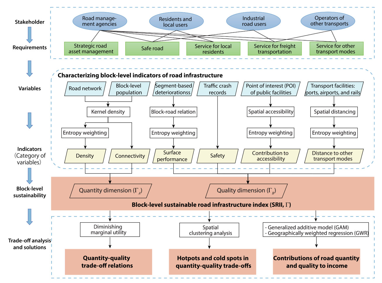
Published reference · STORSTOR paper Fig. 2 — the whole model in one picture, and the plan of §3 of this
page: stakeholder requirements define the variables, entropy weighting builds the quantity
and quality dimensions of the sustainable road infrastructure index (SRII), and three
analyses follow — DMU trade-off relations, hotspot/cold-spot clustering, and the
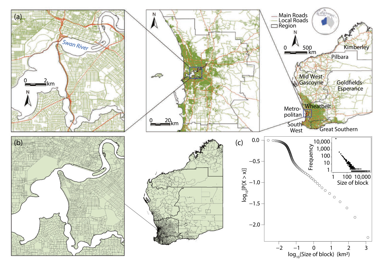
contribution of each dimension to income. Click to enlarge.Published reference · STORSTOR paper Fig. 1 — the published study area: the road network of Western
Australia (a), its 42,425 blocks (b), and the power-law block-size distribution (c). The
demo below replaces this with a simulated 40 × 40 grid so every number on the page
regenerates from the folder.
◆Reader anchor
Two indices per block → one curve between them → the curve's slope names the stage →
the stages plus the cluster overlay name the strategy. ΓA is quantity,
ΓB is quality, u(ΓA) is the LOESS fit of ΓB on
ΓA, η is its slope, and the two boundaries sit at max(η) and at max(u) where
η = 0. Everything on this page serves that line.
✓What you need
R 4.1+ and the folder from the download button. The method itself is
R/02-stor-core.R, about 200 lines of base R with no package dependency —
entropy weights, the LOESS utility (via stats::loess), local Moran's I and
the GWR are all in that one file. mgcv (ships with R) runs the GAM;
ggplot2 and patchwork draw the figures; spdep is used
only by the tests to cross-check the local Moran implementation. The full pipeline runs in
about 20 seconds.
1.2 Method Logic
STOR chains four standard tools into one argument. Each link is simple; the model is the
order they come in:
Utility curveu(ΓA) = LOESS fit of ΓB on
ΓA (Eq. 7)
→
Marginal utilityη = Δu / ΔΓA, a difference quotient of the
fitted curve (Eq. 8–9)
→
DMU stagesIR | MR at max(η) · MR | NR at max(u), where η = 0
→
Trade-off mapsLISA clusters of both dimensions, overlaid; GAM + GWR
contributions to income
Key concepts and equations
Standardization with a sign (Eq. 3). Every indicator is min–max scaled to [0, 1];
indicators where less is better (roughness, crashes, distance to ports) are flipped:
Yj = (Xj − min Xj) / (max Xj − min Xj) (positive) Yj = (max Xj − Xj) / (max Xj − min Xj) (negative)
Entropy weights (Eq. 4–5). Within each indicator category, variables carrying more
variation (lower information entropy) receive larger weights:
Category indices are the entropy-weighted sums (Eq. 6); ΓA and ΓB
average their categories equally, and the SRII Γ averages the two dimensions.
The utility function and its slope (Eq. 7–9). The trade-off relation is the
nonparametric regression of quality on quantity, and the marginal utility is its difference
quotient:
u(ΓA, ΓB) = f(ΓA) (LOESS), η = Δu / ΔΓA
The IR|MR boundary t1 sits at max(η) — quality is still being bought fastest —
and the MR|NR boundary t2 sits at max(u), where η crosses zero for good.
Clusters and contributions. Local Moran's I (LISA) classifies each dimension
into HH / LL clusters at p < 0.05; blocks that are HH (or LL) in both
dimensions are the joint hotspots (cold spots), and the cold-side overlay names a strategy
per block (Fig. 8b of the paper). A GAM (Eq. 10) and a GWR (Eq. 11) then
measure each dimension's contribution to mean income as the deviance explained that is lost
when the dimension is dropped.
1.3 Reproduction Scope
The published case rests on restricted administrative data — road deterioration sensors,
crash records, block-level population — that are not distributed with the article. This
reproduction therefore simulates a study area with a known trade-off hidden inside: an
urbanisation field drives 14 block-level indicators, quality follows a ground-truth utility
curve with boundaries embedded at ΓA = 0.070 and 0.585 (the published values
are 0.072 and 0.585), and income depends on both dimensions with coefficients that drift across
the map. The pipeline is then judged by whether it recovers what the simulation hid —
which is verified by run-all.R test. Everything tagged Demo run regenerates
from this folder; everything tagged Published reference is a static image from the source
article. The demo runs end to end with R 4.6.0.
Item
Demo template
Published reference
Data
1,600 simulated blocks (40 × 40 grid, 10 km cells) with 14
indicators in 6 categories, population and income (data/blocks.csv);
the embedded truth in data/derived/
42,425 blocks of Western Australia; 15 indicators from road, sensor, crash, POI
and census data (paper Table 1)
Method
R/02-stor-core.R — entropy SRII, LOESS utility + marginal utility,
DMU staging, LISA, GWR, in base R
Song et al. (2021) §3, using kernel densities, entropy weighting, LOESS,
LISA, mgcv and spgwr
Results
boundaries t1 = 0.092, t2 = 0.576
recovered against the embedded 0.070 / 0.585; stage agreement 94%; contribution of
ΓB 16.2% vs ΓA 0.4%
t1 = 0.072, t2 = 0.585 (Fig. 6b);
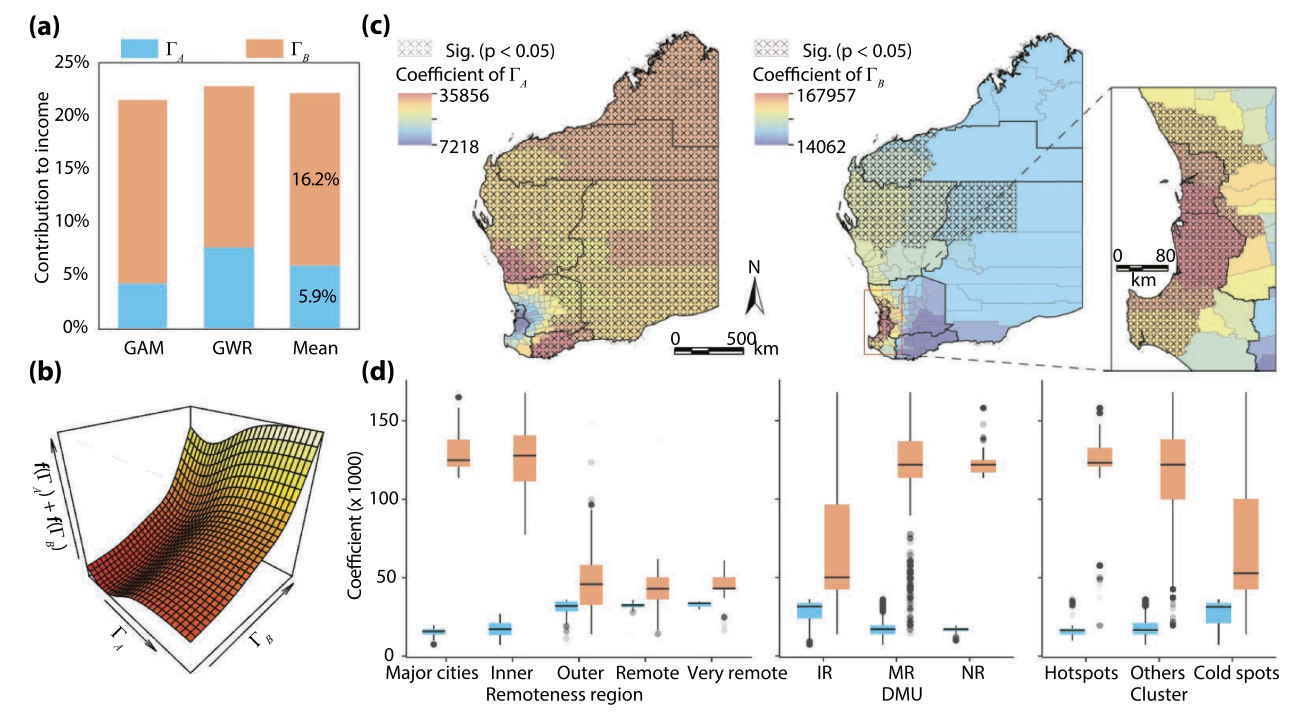
contribution of ΓB 16.2% vs ΓA 5.9% (Fig. 11a)
Figures
fig01–fig05 from R/p01–p05
STOR Figs 1–4 and 6–11, embedded as reference images beside their demo counterparts
What the template regenerates versus what is shown as published reference.
How to use this page
To reproduce the demo: the folder holds the method, the pipeline, the simulation and
the tests. Run Rscript run-all.R test, then Rscript run-all.R.
To use the method on your own problem: §2.2 prints the whole implementation, so you
can paste it into your own script; §2.4 gives the data contract and §4.1 the porting
steps.
To write the paper: §4.2 maps every result file to a manuscript element.
2 Setup, Code & Data
2.1 Environment & Dependencies
The method needs nothing. R/02-stor-core.R is written in base R —
stats::loess included — so source() it and the whole of STOR is
available: index construction, the utility curve, DMU staging, local Moran's I and the GWR.
The pipeline around it uses a few packages, and each step reports and continues if one is
missing.
R console — optional, for the figures and the test cross-check
# Figures
install.packages(c("ggplot2", "patchwork"))

# Tests only: cross-checks the built-in local Moran's I against
# spdep::localmoran() (they agree to 1e-9; skipped when absent)
install.packages("spdep")

# The GAM uses mgcv, which ships with every R installation.
The method is dependency-free by design, so it can be dropped into any project.
!Two deliberate departures from the published pipeline
The paper fitted its GWR with the spgwr package and identified cold-spot
towns through a POI-density aggregation (its Fig. 3) that needs data not distributed
with the article. Here the GWR is re-implemented in base R with an adaptive bisquare kernel
and AICc bandwidth selection — tests/test-01 proves it collapses to global OLS
when every block is co-located — and the town-identification step is simplified to a
per-block development-strategy overlay (§3, Step 4), which preserves the decision logic
of the paper's Fig. 8b without the proprietary POI layer.
2.2 The Method in One File
The whole of STOR is printed here so it can be copied out and used directly; it is also
R/02-stor-core.R in the download, and the two are the same file. Four pieces:
index construction, the trade-off relation, spatial clusters, and the GWR.
Index construction: standardization, entropy weights, SRII
Three small functions build every index. stor_standardize() is Eq. 3 with
the indicator's sign; stor_entropy_weights() is Eq. 4–5 with the two edge
cases (a zero column, a constant column) handled explicitly; stor_srii() assembles
Eq. 6 exactly as the paper weights it — entropy within categories, equal across categories,
equal across the two dimensions.
R/02-stor-core.R — index construction
# -- 1. Index construction ----------------------------------------------------

#' Min-max standardization (Eq. 3). sign = +1 keeps orientation, sign = -1
#' flips it, so that larger standardized values always mean "more sustainable".
stor_standardize <- function(x, sign = +1) {
  rng <- range(x, na.rm = TRUE)
  if (diff(rng) == 0) return(rep(0, length(x)))
  y <- (x - rng[1]) / (rng[2] - rng[1])
  if (sign < 0) y <- 1 - y
  y
}

#' Entropy weights of the columns of a standardized matrix Y (Eq. 4-5).
#' Columns carrying more variation (lower entropy) receive larger weights.
stor_entropy_weights <- function(Y) {
  Y <- as.matrix(Y)
  m <- nrow(Y)
  ent <- apply(Y, 2, function(y) {
    s <- sum(y, na.rm = TRUE)
    if (s == 0) return(1)                     # constant column: no information
    th <- y / s
    th <- th[th > 0]
    -sum(th * log(th)) / log(m)
  })
  phi <- 1 - ent
  if (sum(phi) == 0) return(rep(1 / ncol(Y), ncol(Y)))
  w <- phi / sum(phi)
  names(w) <- colnames(Y)
  w
}

#' Block-level SRII (Eq. 6). `data` holds the raw indicator columns;
#' `indicators` is a data.frame(name, category, dimension, sign) as in the
#' config. Weighting follows the paper: entropy weights within each category,
#' equal weights across categories within a dimension, equal weights across
#' the two dimensions.
#'
#' Returns list(weights, categories, gamma_a, gamma_b, gamma).
stor_srii <- function(data, indicators) {
  Y <- sapply(seq_len(nrow(indicators)), function(j)
    stor_standardize(data[[indicators$name[j]]], indicators$sign[j]))
  colnames(Y) <- indicators$name

  weights <- do.call(rbind, lapply(split(indicators, indicators$category), function(ind) {
    w <- stor_entropy_weights(Y[, ind$name, drop = FALSE])
    data.frame(name = ind$name, category = ind$category[1],
               dimension = ind$dimension[1], weight = as.numeric(w))
  }))
  rownames(weights) <- NULL

  cat_names <- unique(indicators$category)
  categories <- sapply(cat_names, function(cn) {
    w <- weights[weights$category == cn, ]
    as.numeric(Y[, w$name, drop = FALSE] %*% w$weight)
  })

  dim_index <- function(dm) {
    cats <- unique(indicators$category[indicators$dimension == dm])
    rowMeans(categories[, cats, drop = FALSE])
  }
  gamma_a <- dim_index("A")
  gamma_b <- dim_index("B")

  list(weights = weights, categories = as.data.frame(categories),
       gamma_a = gamma_a, gamma_b = gamma_b,
       gamma = (gamma_a + gamma_b) / 2)
}
The trade-off relation: LOESS utility, marginal utility, DMU stages
stor_utility() fits the LOESS on the raw blocks, not on bin means — the
span is a nearest-neighbour fraction, so the bandwidth is automatically narrow where blocks pile
up at low ΓA, exactly where the utility rises fastest. Equal-count bin means are
returned too, but only as the display dots of Fig. 6b. The marginal utility is the
difference quotient of Eq. 9 taken as a centred difference over a small finite
ΔΓA (≈6% of the range), which keeps η from amplifying sub-Δ wiggles of the fitted
curve. stor_dmu() then places t1 at max(η) and t2 at max(u),
where η crosses zero for good.
R/02-stor-core.R — utility function and DMU boundaries
# -- 2. Trade-off relation and diminishing marginal utility -------------------

#' The utility function u(Gamma_A) = f(Gamma_A) with Gamma_B as the observed
#' response (Eq. 7), fitted by LOESS on the raw blocks. The span is a
#' nearest-neighbour fraction, so the bandwidth adapts to the data: narrow
#' where blocks pile up at low Gamma_A — exactly where the utility rises
#' fastest — and wide in the sparse tail. The marginal utility eta is the
#' difference quotient of the fitted curve (Eq. 8-9). Equal-count bin means
#' are also returned; they are the black dots of the paper's Fig. 6b, for
#' display only.
#'
#' Returns list(bins, curve) where curve has columns ga, u, eta.
stor_utility <- function(gamma_a, gamma_b, n_bins = 40, span = 0.2,
                         n_eval = 200) {
  brk <- unique(stats::quantile(gamma_a, seq(0, 1, length.out = n_bins + 1)))
  bin <- cut(gamma_a, brk, include.lowest = TRUE)
  bins <- data.frame(
    ga = tapply(gamma_a, bin, mean),
    gb = tapply(gamma_b, bin, mean),
    n  = as.numeric(table(bin))
  )
  bins <- bins[bins$n > 0, ]

  fit <- stats::loess(gb ~ ga, data = data.frame(ga = gamma_a, gb = gamma_b),
                      span = span, degree = 2, family = "gaussian",
                      control = stats::loess.control(surface = "direct"))

  ga_eval <- seq(min(gamma_a), max(gamma_a), length.out = n_eval)
  u  <- stats::predict(fit, data.frame(ga = ga_eval))
  se <- stats::predict(fit, data.frame(ga = ga_eval), se = TRUE)$se.fit

  # Difference quotient of Eq. 9 as a centred difference over a small but
  # finite Delta Gamma_A (about 6% of the observed range), which keeps eta
  # from amplifying sub-Delta wiggles of the fitted curve.
  w <- max(1L, round(n_eval * 0.03))
  idx <- seq_len(n_eval)
  lo <- pmax(idx - w, 1L); hi <- pmin(idx + w, n_eval)
  eta <- (u[hi] - u[lo]) / (ga_eval[hi] - ga_eval[lo])

  list(bins = bins, fit = fit,
       curve = data.frame(ga = ga_eval, u = u, se = se, eta = eta))
}

#' DMU stage boundaries on a fitted utility curve. The IR-MR boundary t1 sits
#' at the maximum marginal utility; the MR-NR boundary t2 sits where the
#' utility peaks — max(u), the point where eta crosses zero for good
#' (Section 3.2 of the paper).
#'
#' Returns list(t1, t2, stage_of) where stage_of(ga) classifies values.
stor_dmu <- function(curve) {
  eta <- curve$eta[-nrow(curve)]
  ga  <- curve$ga[-nrow(curve)]

  i1 <- which.max(eta)
  t1 <- ga[i1]

  u <- curve$u[-nrow(curve)]
  i2 <- max(which.max(u), i1 + 1)
  t2 <- ga[i2]

  stage_of <- function(x)
    factor(ifelse(x < t1, "IR", ifelse(x < t2, "MR", "NR")),
           levels = c("IR", "MR", "NR"))

  list(t1 = t1, t2 = t2, i1 = i1, i2 = i2, stage_of = stage_of)
}
Spatial clusters: local Moran's I and the trade-off overlay
Local Moran's I with conditional-permutation pseudo p-values, on a queen-contiguity
neighbour list, in ~40 lines. tests/test-01 verifies the statistic against
spdep::localmoran() to 1e-9, so nothing is lost by not depending on the package.
stor_tradeoff_groups() is the overlay of the paper's §3.3: HH ∩ HH →
hotspot, LL ∩ LL → cold spot, and each cold-side block gets the development strategy
of Fig. 8b — more quantity, more quality, or both.
R/02-stor-core.R — LISA and the trade-off overlay
# -- 3. Spatial clusters (LISA) -----------------------------------------------

#' Queen-contiguity neighbours on a regular grid of blocks. `col` and `row`
#' are integer grid positions. Returns a list of integer index vectors.
stor_grid_neighbors <- function(col, row) {
  n <- length(col)
  key <- paste(col, row)
  idx <- seq_len(n)
  lookup <- new.env(hash = TRUE, size = n)
  for (i in idx) assign(key[i], i, envir = lookup)
  lapply(idx, function(i) {
    nb <- integer(0)
    for (dc in -1:1) for (dr in -1:1) {
      if (dc == 0 && dr == 0) next
      k <- paste(col[i] + dc, row[i] + dr)
      j <- lookup[[k]]
      if (!is.null(j)) nb <- c(nb, j)
    }
    sort(nb)
  })
}

#' Local Moran's I with conditional-permutation pseudo p-values (Anselin 1995).
#' `nb` is a neighbour list as returned by stor_grid_neighbors(); weights are
#' row-standardized. Matches spdep::localmoran() on Ii (the tests check this).
stor_local_moran <- function(x, nb, nsim = 999, seed = NULL) {
  if (!is.null(seed)) set.seed(seed)
  n <- length(x)
  z <- x - mean(x)
  s2 <- sum(z^2) / n
  lag <- vapply(seq_len(n), function(i) mean(z[nb[[i]]]), numeric(1))
  Ii <- z / s2 * lag

  p <- vapply(seq_len(n), function(i) {
    k <- length(nb[[i]])
    if (k == 0) return(NA_real_)
    zi <- z[-i]
    perm <- vapply(seq_len(nsim), function(s)
      z[i] / s2 * mean(sample(zi, k)), numeric(1))
    (1 + sum(abs(perm) >= abs(Ii[i]))) / (1 + nsim)
  }, numeric(1))

  data.frame(Ii = Ii, z = z, lag = lag, p = p)
}

#' HH / LL / HL / LH / Not significant labels from a local Moran result.
stor_lisa_class <- function(lm_res, alpha = 0.05) {
  cl <- rep("Not significant", nrow(lm_res))
  sig <- !is.na(lm_res$p) & lm_res$p < alpha
  cl[sig & lm_res$z > 0 & lm_res$lag > 0] <- "HH"
  cl[sig & lm_res$z < 0 & lm_res$lag < 0] <- "LL"
  cl[sig & lm_res$z > 0 & lm_res$lag < 0] <- "HL"
  cl[sig & lm_res$z < 0 & lm_res$lag > 0] <- "LH"
  factor(cl, levels = c("HH", "LL", "HL", "LH", "Not significant"))
}

#' Overlay the quantity and quality cluster labels (Section 3.3): a block is a
#' trade-off hotspot when both dimensions are HH, a cold spot when both are
#' LL. Cold-side blocks are also assigned a development strategy, following
#' Fig. 8b: a quantity-only cold spot calls for more quantity, a quality-only
#' cold spot for more quality, a joint cold spot for both.
stor_tradeoff_groups <- function(class_a, class_b) {
  cluster <- rep("Others", length(class_a))
  cluster[class_a == "HH" & class_b == "HH"] <- "Hotspot"
  cluster[class_a == "LL" & class_b == "LL"] <- "Cold spot"

  strategy <- rep("No cold spot", length(class_a))
  strategy[class_a == "LL" & class_b != "LL"] <- "Increase quantity"
  strategy[class_a != "LL" & class_b == "LL"] <- "Increase quality"
  strategy[class_a == "LL" & class_b == "LL"] <- "Increase both"

  data.frame(cluster = factor(cluster, c("Hotspot", "Others", "Cold spot")),
             strategy = factor(strategy, c("Increase quantity", "Increase both",
                                           "Increase quality", "No cold spot")))
}
Geographically weighted regression
A location-wise weighted least squares with an adaptive bisquare kernel (Eq. 11): the
bandwidth at each block is the distance to its k-th neighbour, and k is chosen by AICc across
the candidates in the config. The hat values are collected during the same pass, so the AICc
costs nothing extra.
R/02-stor-core.R — GWR with adaptive bandwidth
# -- 4. Geographically weighted regression ------------------------------------

#' GWR with an adaptive bisquare kernel (Eq. 11). `k` is the number of
#' neighbours defining the local bandwidth. Returns location-wise coefficients,
#' fitted values, R2 and the AICc used for bandwidth selection.
stor_gwr <- function(y, X, coords, k) {
  X <- cbind(Intercept = 1, as.matrix(X))
  n <- nrow(X); p <- ncol(X)
  coords <- as.matrix(coords)
  beta <- matrix(NA_real_, n, p, dimnames = list(NULL, colnames(X)))
  fitted <- numeric(n)
  hat <- numeric(n)

  for (i in seq_len(n)) {
    d <- sqrt((coords[, 1] - coords[i, 1])^2 + (coords[, 2] - coords[i, 2])^2)
    h <- sort(d)[min(k, n)]
    w <- if (h > 0) ifelse(d < h, (1 - (d / h)^2)^2, 0) else rep(1, n)
    XtW <- t(X * w)
    XtWXi <- solve(XtW %*% X)
    bi <- XtWXi %*% (XtW %*% y)
    beta[i, ] <- bi
    fitted[i] <- X[i, ] %*% bi
    hat[i] <- (X[i, , drop = FALSE] %*% XtWXi %*% XtW)[i]
  }

  res <- y - fitted
  rss <- sum(res^2)
  r2 <- 1 - rss / sum((y - mean(y))^2)
  tr_s <- sum(hat)
  sigma2 <- rss / n
  aicc <- n * log(2 * pi * sigma2) + n * (n + tr_s) / (n - 2 - tr_s)

  list(beta = as.data.frame(beta), fitted = fitted, residuals = res,
       r2 = r2, aicc = aicc, tr_s = tr_s, k = k)
}

#' Adaptive bandwidth selection: fit at each candidate k, keep the lowest AICc.
stor_gwr_select <- function(y, X, coords, ks) {
  fits <- lapply(ks, function(k) stor_gwr(y, X, coords, k))
  aicc <- vapply(fits, `[[`, numeric(1), "aicc")
  best <- which.min(aicc)
  out <- fits[[best]]
  out$candidates <- data.frame(k = ks, aicc = aicc,
                               r2 = vapply(fits, `[[`, numeric(1), "r2"))
  out
}
2.3 Project Structure & Configuration
One folder, one config, one command. Steps write to data/, results/,
tables/ and figs/; each step reads what the previous one wrote, so a
single step can be re-run after a config change without repeating the whole pipeline.
folder layout
STOR/
├── run-all.R                  # one command reproduces everything
├── config/project-config.R    # the ONLY file you edit when porting
├── R/
│   ├── 00-config.R            # paths and result-file names
│   ├── 01-helpers.R           # logging, IO, figure helpers
│   ├── 02-stor-core.R         # THE METHOD (base R, standalone)
│   ├── 10-simulate-data.R     # replace this step with your own data
│   ├── 20-srii.R              # entropy-weighted indices
│   ├── 30-dmu.R               # utility curve + DMU stages
│   ├── 40-lisa.R              # clusters + trade-off groups
│   ├── 50-income-models.R     # GAM + GWR contributions
│   ├── 90-tables.R            # LaTeX tables
│   └── p01–p05 ...            # the five figures
├── data/                      # blocks.csv + derived/ (embedded truth)
├── results/  tables/  figs/   # regenerated outputs
├── tests/                     # the two verification scripts
└── env/                       # requirements + session-info.txt
The config carries the project identity, the indicator table (which column belongs to which
category, dimension and sign — the analogue of the paper's Table 1), the simulation's
ground truth, and every analysis constant:
config/project-config.R — the only file you edit
# =============================================================================
# project-config.R — the ONLY file you edit when porting this template
#                    to a new domain.
# =============================================================================
# Everything below is read by R/00-config.R and used by every pipeline step.
# After editing this file, run:  Rscript run-all.R
# =============================================================================


# -- 1. Project identity ------------------------------------------------------
PROJECT_ID     <- "stor-demo"
PROJECT_TITLE  <- "Spatial trade-off relation between [QUANTITY] and [QUALITY] in [YOUR STUDY AREA]"
DOMAIN         <- "sustainable road infrastructure (simulated blocks)"
TARGET_JOURNAL <- "TBD"


# -- 2. Input data ------------------------------------------------------------
# The method needs ONE table: spatial units (blocks) with indicator variables.
# Each indicator belongs to a category, each category to a dimension (quantity
# A or quality B), and each carries a sign: +1 if more of it means more
# sustainable, -1 otherwise (Table 1 of the paper).

BLOCK_FILE <- "data/blocks.csv"

XCOL <- "x_km"                 # block centroid coordinates, km
YCOL <- "y_km"

# name = column in BLOCK_FILE; category groups variables for entropy weighting;
# dimension assigns the category to quantity (A) or quality (B).
INDICATORS <- data.frame(
  name = c("road_density", "main_road_density", "roads_per_person",
           "intersection_density",
           "roughness", "rutting", "deflection", "curvature",
           "crash_rate",
           "craf_schools", "craf_hospitals", "craf_industry",
           "dist_ports", "dist_airports"),
  category = c("density", "density", "density",
               "connectivity",
               "performance", "performance", "performance", "performance",
               "safety",
               "accessibility", "accessibility", "accessibility",
               "transport_modes", "transport_modes"),
  dimension = c("A", "A", "A", "A",
                "B", "B", "B", "B", "B",
                "B", "B", "B", "B", "B"),
  sign = c(+1, +1, +1, +1,
           -1, -1, -1, -1,
           -1,
           +1, +1, +1,
           -1, -1),
  stringsAsFactors = FALSE
)


# -- 3. Simulation ------------------------------------------------------------
# Only used by R/10-simulate-data.R. Replace that step with your own data and
# nothing here matters.
GRID_NX <- 40                  # blocks west-east
GRID_NY <- 40                  # blocks south-north
CELL_KM <- 10                  # block size, km

# Ground-truth utility curve embedded in the simulation. The logistic rise
# puts the maximum marginal utility at TRUE_T1; the slow linear gain keeps the
# curve climbing through the MR stage; the penalty beyond TRUE_T2 turns it
# down, so eta = 0 near TRUE_T2. The published case found t1 = 0.072 and
# t2 = 0.585 (Fig. 6b of Song et al. 2021).
TRUE_T1   <- 0.07              # IR -> MR boundary on Gamma_A
TRUE_T2   <- 0.585             # MR -> NR boundary on Gamma_A
U_BASE    <- 0.57              # utility at Gamma_A = 0
U_AMP     <- 0.20              # size of the logistic rise
U_SLOPE   <- 0.032             # logistic scale (smaller = steeper rise)
U_LIN     <- 0.10              # linear gain through the MR stage
U_DECLINE <- 0.80              # decline rate past TRUE_T2 (power 1.5)


# -- 4. Trade-off relation (LOESS + marginal utility) -------------------------
N_BINS     <- 40               # equal-count Gamma_A bins (display dots only)
LOESS_SPAN <- 0.15             # LOESS nearest-neighbour fraction, raw blocks
N_EVAL     <- 200              # evaluation points for u() and eta


# -- 5. Spatial clusters (LISA) -----------------------------------------------
LISA_NSIM  <- 999              # conditional permutations for pseudo p-values
LISA_ALPHA <- 0.05             # significance level for HH / LL clusters


# -- 6. Income contribution (GAM + GWR) ---------------------------------------
INCOME_COL   <- "income"       # response, 1000 $ per person, in BLOCK_FILE
GWR_NEIGHBORS <- c(40, 60, 80, 100, 150)   # adaptive bandwidth candidates
SEED <- 100


# -- 7. Figure style ----------------------------------------------------------
FIG_WIDTH_SINGLE <- 9
FIG_WIDTH_DOUBLE <- 19
FIG_DPI          <- 600
FIG_DEVICES      <- c("pdf", "png")

PALETTE_DMU  <- c(IR = "#74C7E8", MR = "#F2C14E", NR = "#F25C54")
PALETTE_DIM  <- c(Gamma_A = "#56B4E9", Gamma_B = "#F08A5D", Gamma = "#4CAF6E")
PALETTE_LISA <- c("Hotspot" = "#B2182B", "Cold spot" = "#2166AC",
                  "Others" = "#D9D9D9")
PALETTE_SEQ  <- c("#2C3E8C", "#3FA0C0", "#8CD07C", "#F2E34C", "#E8A03C",
                  "#C0503C")
2.4 Data Contract
The method needs one table: spatial units with indicator columns. Coordinates are
planar (km in the demo); on real data any projected CRS works. The indicator table in the
config declares everything else — which columns exist, how they group, and which direction is
"better".
Column(s) in data/blocks.csv
Category
Dimension
Sign
Published analogue (Table 1)
road_density, main_road_density, roads_per_person
density
ΓA
+
road density; main-road density; roads shared by population
intersection_density
connectivity
ΓA
+
road intersection density
roughness, rutting, deflection, curvature
performance
ΓB
−
deterioration sensor variables (0.786 M observations)
crash_rate
safety
ΓB
−
crashes per million vehicles, 2015–2019
craf_schools, craf_hospitals, craf_industry
accessibility
ΓB
+
CRAF = dGeometric / dNetwork to five facility types (Eq. 1–2)
dist_ports, dist_airports
transport_modes
ΓB
−
network distance to ports, airports, railways
x_km, y_km; col, row
block centroids; integer grid position (queen contiguity)
block polygons and their contiguity
population, income
residents per block; mean income, 1000 $ per person
ABS population grid; LGA mean income
The demo's 14 indicators against the paper's Table 1. The CRAF ratio is
dimensionless in (0, 1]: geometric distance over shortest network distance, so 1 means the
road network is a straight-line-perfect connection.
◆What the simulation embeds — and why that is the point
An urbanisation field (a main city, a secondary town, smooth spatial noise) drives all
four quantity indicators. Quality follows the ground-truth curve of the config — a logistic
rise with maximum slope at ΓA = 0.070, a slow linear gain through MR,
and a decline past 0.585 — plus a spatially smooth quality field that quantity knows nothing
about. Income pays for quality about ten times what it pays for quantity, with the quality
coefficient drifting northward. Every one of those choices is a recoverable target:
data/derived/simulation-truth.csv stores the latent fields, and §3.2 checks the
pipeline finds them.
3 Reproduction Pipeline, Results & Validation
3.1 Pipeline Execution
One command reproduces everything; the arguments select subsets when iterating:
shell — from the STOR/ folder root
Rscript run-all.R          # full pipeline: steps 10-90 + the five figures  (~20 s)
Rscript run-all.R test     # only the verification tests                    (~5 s)
Rscript run-all.R 30       # re-run one step, e.g. the DMU analysis
Rscript run-all.R figures  # only the figure scripts
==================================================================
Project : stor-demo
Domain : sustainable road infrastructure (simulated blocks)
==================================================================
== 10 Simulate block data (40 x 40 blocks) ==============
wrote data/blocks.csv (1600 rows)
wrote data/derived/simulation-truth.csv (1600 rows)
embedded DMU boundaries: t1 = 0.070, t2 = 0.585
== 20 SRII: entropy-weighted indices ====================
wrote results/entropy-weights.csv (14 rows)
wrote results/srii-blocks.csv (1600 rows)
Gamma_A mean 0.326 (sd 0.210), Gamma_B mean 0.517 (sd 0.137)
category accessibility weights: 0.31 0.35 0.34
category connectivity weights: 1.00
category density weights: 0.34 0.33 0.33
category performance weights: 0.27 0.26 0.23 0.24
category safety weights: 1.00
category transport_modes weights: 0.47 0.53
== 30 DMU: utility curve and stage boundaries ===========
wrote results/utility-bins.csv (40 rows)
wrote results/utility-curve.csv (200 rows)
wrote results/dmu-boundaries.csv (2 rows)
wrote results/dmu-stages.csv (1600 rows)
t1 = 0.092 (max eta), t2 = 0.576 (eta = 0); embedded truth 0.070 / 0.585
blocks per stage: IR 205, MR 1162, NR 233
== 40 LISA: clusters and trade-off groups ===============
wrote results/lisa-clusters.csv (1600 rows)
wrote results/tradeoff-groups.csv (5 rows)
clusters: Hotspot 117, Others 1241, Cold spot 242
strategies (cold-side blocks): Increase quantity 181, Increase both 242, Increase quality 49, No cold spot 1128
== 50 GAM + GWR: income contribution ====================
GAM deviance explained 47.0% (Gamma_A 0.6%, Gamma_B 28.1%)
GWR (adaptive k = 80) R2 0.939 (Gamma_A 0.2%, Gamma_B 4.3%)
wrote results/income-contribution.csv (6 rows)
wrote results/gwr-coefficients.csv (1600 rows)
GWR bandwidth candidates: k=40 AICc=6200.7; k=60 AICc=6169.9; k=80 AICc=6167.3; k=100 AICc=6175.1; k=150 AICc=6206.1
== 90 Tables ============================================
wrote tables/table-entropy-weights.tex
wrote tables/table-dmu-stages.tex
wrote tables/table-tradeoff-strategies.tex
wrote tables/table-income-contribution.tex
wrote figs/fig01-srii-maps.{pdf,png}
wrote figs/fig02-dmu-tradeoff.{pdf,png}
wrote figs/fig03-dmu-stages.{pdf,png}
wrote figs/fig04-lisa-tradeoff.{pdf,png}
wrote figs/fig05-income-contribution.{pdf,png}
==================================================================
Finished in 17.8 s
Outputs: results/ tables/ figs/ data/
3.2 Recover the Embedded Truth
The simulation knows its own answers, so the tests are sharp: not "does it run" but "does the
pipeline find what was hidden". Two scripts, 25 checks. test-01 proves the
implementation satisfies the definitions — entropy weight axioms, the DMU boundary conditions,
local Moran's I against spdep, the GWR against OLS. test-02
proves the analysis recovers the simulation — the boundaries, the stages, the clusters, the
income attribution.
Quantity
Embedded truth
Recovered
Check
IR | MR boundary t1
0.070
0.092
within 0.05 — pass
MR | NR boundary t2
0.585
0.576
within 0.08 — pass
DMU stage of each block
—
94% agreement
> 85% — pass
ΓA vs latent quantity
—
r = 0.998
> 0.95 — pass
ΓB vs latent quality
—
r = 0.986
> 0.90 — pass
Contribution to income
quality ≫ quantity
ΓB 16.2% vs ΓA 0.4%
ΓB > ΓA — pass
Northward drift of the quality coefficient
βB: 35 → 55
r = 0.55 with the GWR surface
> 0.5 — pass
The headline recoveries. The published case sits nearby: t1 = 0.072,
t2 = 0.585, and a mean ΓB contribution of 16.2% against 5.9% for
ΓA (paper Figs. 6b, 11a).
==================================================================
Project : stor-demo
Domain : sustainable road infrastructure (simulated blocks)
==================================================================
== test-01 Method properties =============================================
standardized values lie in [0, 1] pass
negative sign flips the orientation pass
entropy weights sum to 1 pass
entropy weights are non-negative pass
higher-variation column gets the larger weight pass
Gamma_A, Gamma_B and Gamma lie in [0, 1] pass
Gamma is the mean of the two dimensions pass
weights sum to 1 within every category pass
t1 sits at the maximum marginal utility pass
t2 sits at the utility maximum, after t1 pass
eta changes sign around t2 (positive before, negative after) pass
stage classifier respects the boundaries pass
local Moran Ii matches spdep (max diff 8.88e-16) pass
local Moran pseudo p-values lie in (0, 1] pass
co-located GWR equals global OLS (max diff 1.76e-12) pass
local GWR fits at least as well as OLS pass
-- 16/16 checks passed --
== test-02 Recover the simulated ground truth ============================
Gamma_A tracks latent quantity (r = 0.998) pass
Gamma_B tracks latent quality (r = 0.986) pass
t1 = 0.092 is within 0.05 of the embedded 0.070 pass
t2 = 0.576 is within 0.08 of the embedded 0.585 pass
stage labels agree with the truth (97%) pass
hotspots are urban blocks (mean urbanisation > 1.5x overall) pass
cold spots are remote blocks (below-average urbanisation) pass
quality contributes more than quantity (16.2% vs 0.4%) pass
GWR recovers the northward drift of beta_B (r = 0.55) pass
-- 9/9 checks passed --
==================================================================
Finished in 0.8 s
Outputs: results/ tables/ figs/ data/
✓Why t1 is recovered less exactly than t2
t2 is the location of a smooth maximum, which LOESS finds robustly.
t1 is the location of the steepest slope of a rise that occupies a tenth of the
ΓA axis; any smoothing spreads that rise, and the spatially correlated quality
field can lean on it locally. With 1,600 blocks the recovered 0.092 sits 0.022 from the
embedded 0.070 — and the same limitation applies to real data, which is worth a sentence in
any manuscript using DMU boundaries for policy.
3.3 Core Analytical Steps
Step 1
Simulate a study area with a known trade-off inside
What this step does
A 40 × 40 grid of 10 km blocks. An urbanisation field — one main city, one
secondary town, smooth spatial noise — is pushed through a rank-based Beta transform, so the
quantity latent keeps the spatial pattern but gains the right-skewed, full-range distribution
of the paper's Fig. 6a. Quality is the ground-truth utility curve of the config applied
to that latent, plus a smooth quality field of its own. Fourteen indicators, population and
income are then generated per block. On real data this whole step is replaced by loading
data/blocks.csv.
Code
R/10-simulate-data.R — the embedded utility curve
# Rank-based Beta transform: keeps the spatial pattern (city gradient, smooth
# noise) but gives quantity a right-skewed distribution with support on the
# whole [0, 1] range, as in Fig. 6a of the paper.
q_true <- stats::qbeta((rank(U + rnorm(n, 0, 0.02)) - 0.5) / n, 1.15, 2.6)

# The ground truth the pipeline must recover: a logistic rise with maximum
# slope at TRUE_T1, a slow linear gain through MR, a decline past TRUE_T2.
u_true <- function(t)
  U_BASE + U_AMP * stats::plogis((t - TRUE_T1) / U_SLOPE) + U_LIN * t -
  U_DECLINE * pmax(t - TRUE_T2, 0)^1.5

qual_true <- u_true(q_true) + 0.05 * smooth_field(2.5) + rnorm(n, 0, 0.012)

beta_a <- 0.5 + 1.0 * g$x_km / max(g$x_km)   # quantity payoff grows eastward
beta_b <- 35  + 20  * g$y_km / max(g$y_km)   # quality payoff grows northward
blocks$income <- 38 + beta_a * q_true + beta_b * qual_true + rnorm(n, 0, 1.5)
Example output
== 10 Simulate block data (40 x 40 blocks) ==============
wrote data/blocks.csv (1600 rows)
wrote data/derived/simulation-truth.csv (1600 rows)
embedded DMU boundaries: t1 = 0.070, t2 = 0.585
◆How to read this result
The truth is planted, so the pipeline can be graded. The boundaries written to simulation-truth.csv — t1 = 0.070, t2 = 0.585 — are what Step 3 has to recover without being told. On real data nothing is planted and this step is one read.csv().
Skew is a modelling choice, not noise. The Beta transform keeps the city gradient but pushes most blocks to low quantity, matching Fig. 6a. A symmetric quantity latent would put too few blocks below t1 for the IR stage to be estimable.
Step 2
Entropy-weighted quantity and quality indices (Eq. 3–6)
What this step does
One call does the index work: stor_srii(blocks, INDICATORS) standardizes
every indicator with its sign, computes entropy weights within each of the six categories,
and assembles ΓA, ΓB and Γ per block. The weights land in
results/entropy-weights.csv — the analogue of the paper's Table 2 — and
the block-level indices in results/srii-blocks.csv.
Code
R/20-srii.R — the entire analytical content of the step
== 20 SRII: entropy-weighted indices ====================
Gamma_A mean 0.331 (sd 0.219), Gamma_B mean 0.500 (sd 0.136)
category density weights: 0.34 0.33 0.33
category performance weights: 0.27 0.26 0.23 0.24
category accessibility weights: 0.31 0.35 0.34
category transport_modes weights: 0.47 0.53
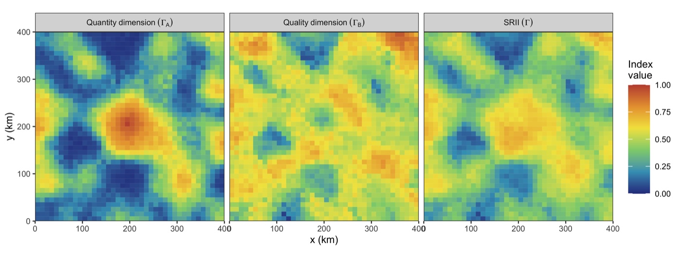
Demo run · fig01Demo fig01 — block-level ΓA, ΓB and Γ on the simulated
grid. Quantity concentrates at the central city and the south-eastern town; quality is
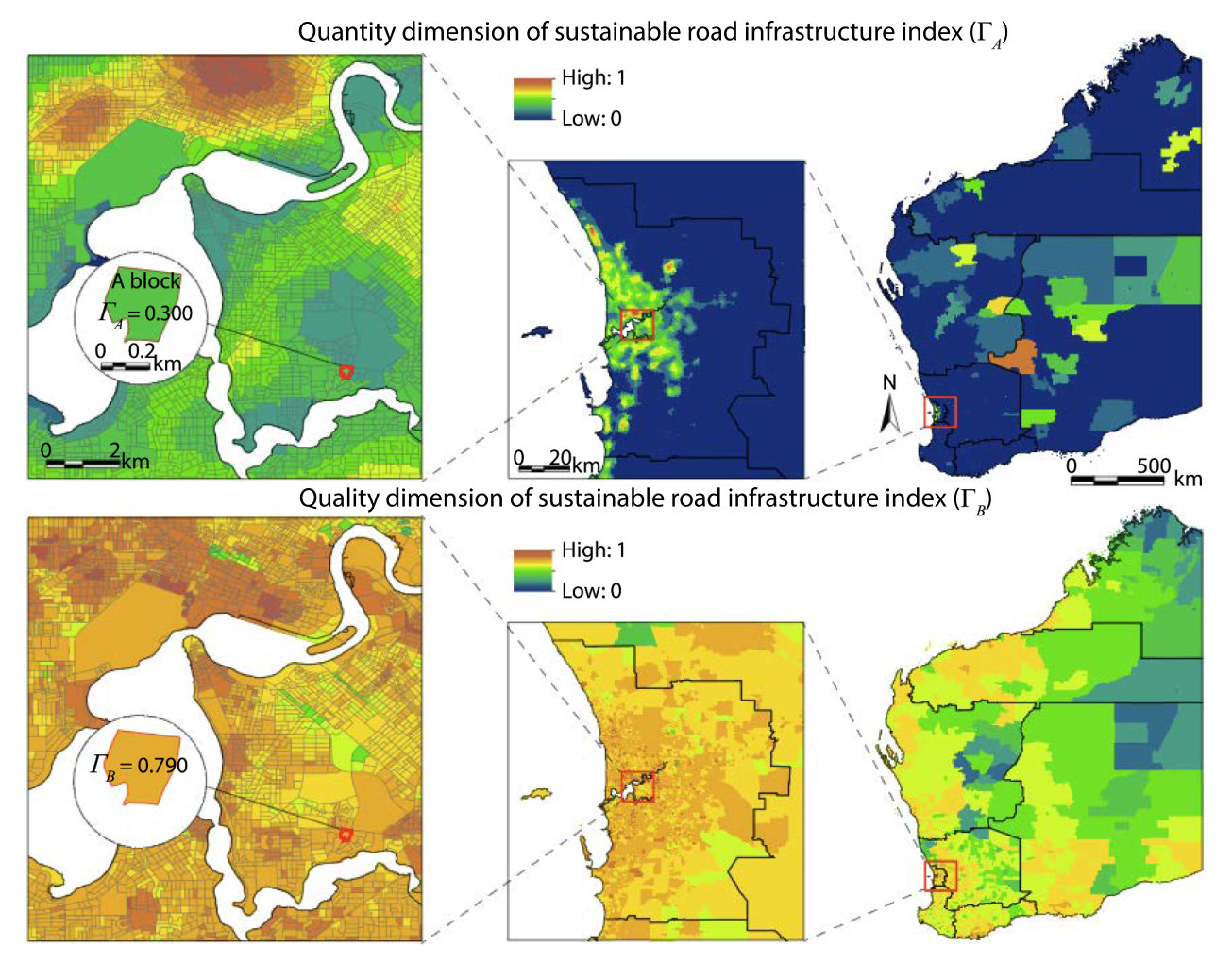
high almost everywhere quantity is moderate, and carries its own smooth field.Published reference · STORSTOR paper Fig. 4 — the published ΓA (top) and ΓB
(bottom) across Western Australia at three zooms. The same structure appears: quantity
is metropolitan, quality is broad with regional texture.
◆How to read this result
Entropy weights are computed within categories, not across them. Each category's weights sum to one, so a category with four indicators does not outvote one with two. This is why the printed weights sit near 1/ncategory rather than near 1/14.
ΓA and ΓB are not interchangeable. Quantity has the larger spread (sd 0.219 against 0.136) because supply is concentrated while quality is diffuse — the asymmetry the whole trade-off analysis rests on.
Step 3
The utility curve, marginal utility and DMU stages (Eq. 7–9)
What this step does
The model's namesake result. stor_utility() fits u(ΓA) by LOESS on
the 1,600 raw blocks; stor_dmu() reads t1 from max(η) and
t2 from max(u); each block is then classified IR / MR / NR by its
ΓA.
Code
R/30-dmu.R — the entire analytical content of the step
== 30 DMU: utility curve and stage boundaries ===========
t1 = 0.092 (max eta), t2 = 0.576 (eta = 0); embedded truth 0.070 / 0.585
blocks per stage: IR 205, MR 1162, NR 233
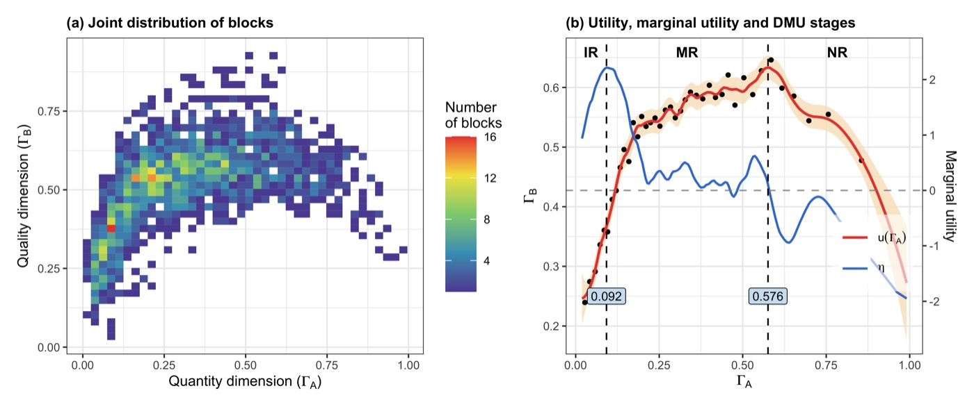
Demo run · fig02Demo fig02 — (a) the joint distribution of the 1,600 blocks and (b) the
recovered relation: LOESS utility (red) with its 95% band, marginal utility (blue), the
bin-mean dots, and the boundaries at ΓA = 0.092 and 0.576 against
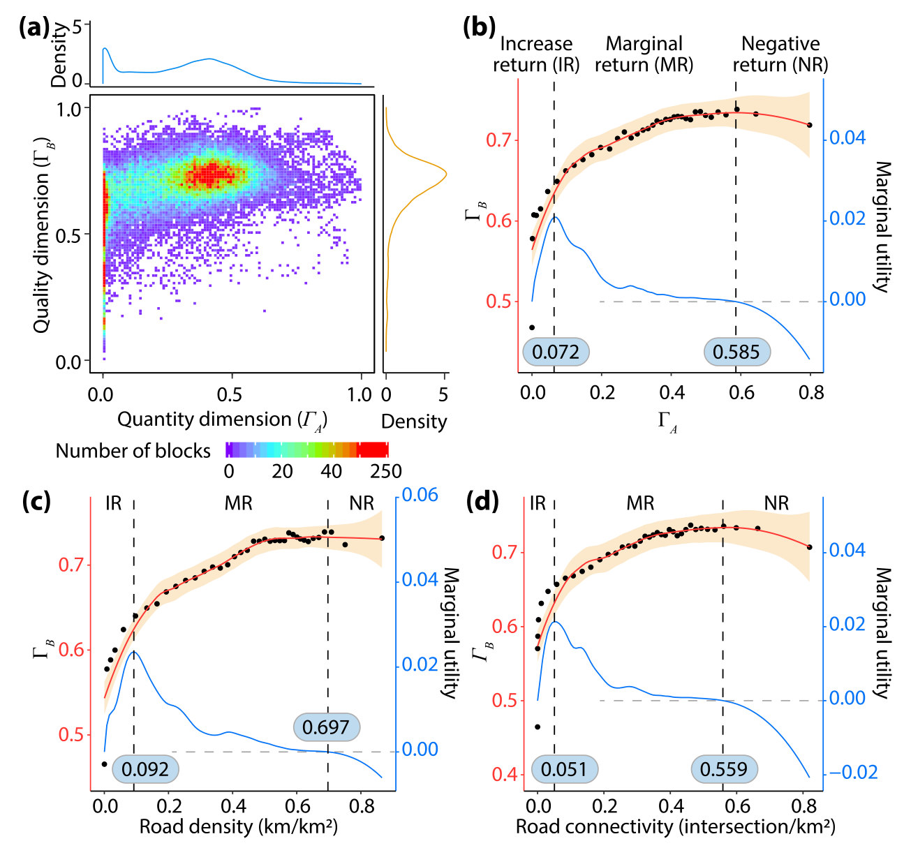
the embedded 0.070 / 0.585.Published reference · STORSTOR paper Fig. 6 — the model's core figure. (a) the joint distribution over
42,425 blocks; (b) the utility and marginal utility with boundaries at 0.072 and 0.585;
(c–d) the same analysis on single indicators. The demo reproduces panel (b)'s logic
exactly and panel (a)'s as a hex-bin.
Read the pair left to right: the demo recovers a curve it can be
graded on (the truth is known), and the published panel shows the same three-stage anatomy
found in real infrastructure — a steep early rise, a long flat middle, a downturn past the
utility peak.
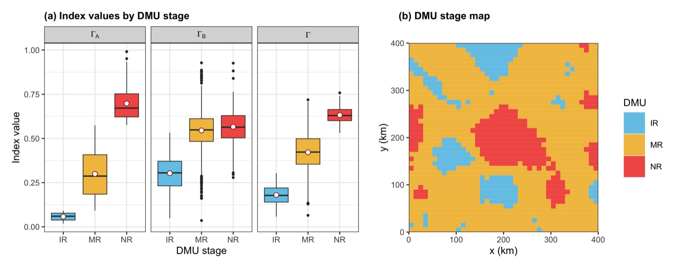
Demo run · fig03Demo fig03 — index distributions by stage and the stage map: IR is remote
(low ΓA, low-mid ΓB), NR rings the city, MR is everything between —
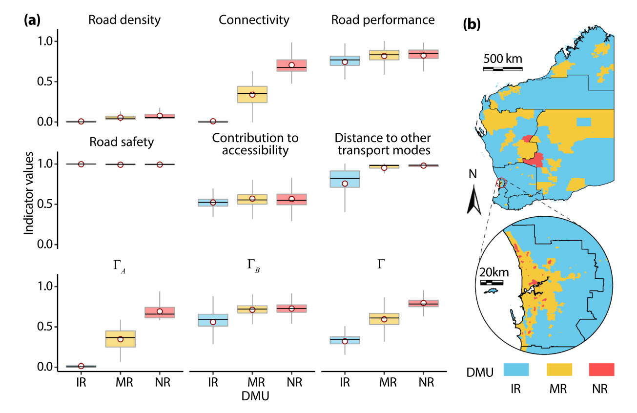
the same ordering as the published Fig. 7.Published reference · STORSTOR paper Fig. 7 — indicator profiles at each DMU stage (a) and the WA
stage map (b): IR dominates the remote interior, MR the settled band, NR the
metropolitan core.
◆How to read this result
The recovered boundaries are the accuracy check. t1 = 0.092 against an embedded 0.070, t2 = 0.576 against 0.585: the LOESS fit finds the downturn precisely and the early inflection approximately, which is the expected asymmetry — max(η) sits on a steep, sparsely-sampled part of the curve.
MR holds most of the blocks by construction. 1,162 of 1,600 fall between the two boundaries. A stage split far from this shape usually means the LOESS span is wrong for your sample size, not that the area has no middle stage.
Step 4
Hotspots, cold spots and trade-off strategies (§3.3 of the paper)
What this step does
Local Moran's I runs on each dimension separately (999 conditional permutations,
p < 0.05), and the overlay makes the trade-off spatial: blocks LL in both
dimensions are joint cold spots; blocks LL in only one dimension name their own remedy.
That per-block strategy map is the demo's stand-in for the paper's cold-spot town
identification (its Fig. 3), which additionally aggregates blocks into towns using a
POI-density layer not distributed with the article.
Code
R/40-lisa.R — the entire analytical content of the step
== 40 LISA: clusters and trade-off groups ===============
clusters: Hotspot 117, Others 1241, Cold spot 242
strategies (cold-side blocks): Increase quantity 181, Increase both 242,
Increase quality 49, No cold spot 1128
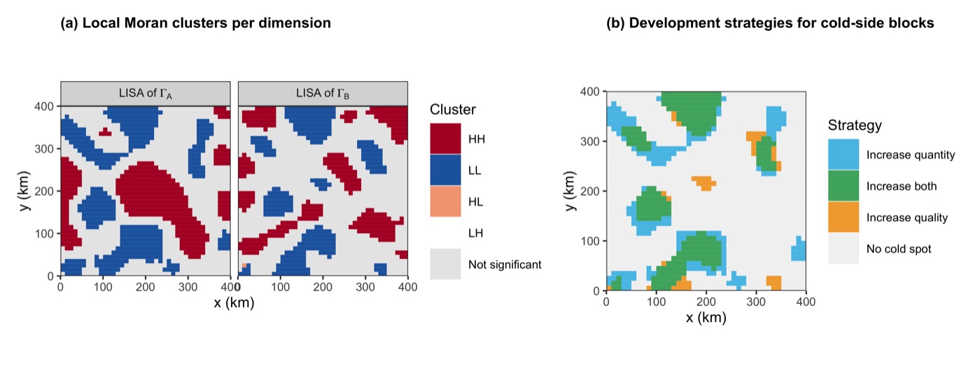
Demo run · fig04Demo fig04 — LISA classes per dimension (a) and the strategy overlay (b):
181 blocks need quantity, 49 need quality, 242 need both. The joint hotspots ring the
city rather than covering its core — the NR downturn keeps the most urban blocks out of
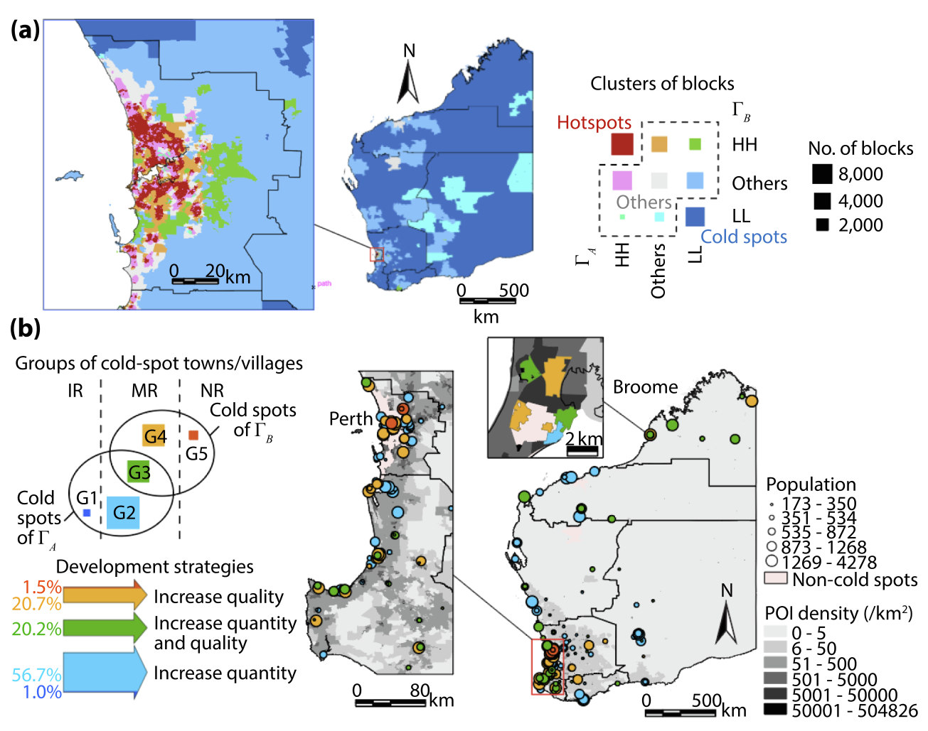
the quality hotspot, which is the trade-off made visible.Published reference · STORSTOR paper Fig. 8 — the published overlay: joint clusters of ΓA
and ΓB (a) and the five cold-spot town groups G1–G5 with their development
strategies (b) — 56.7% of cold-spot towns need quantity, 20.7% quality, 20.2% both.
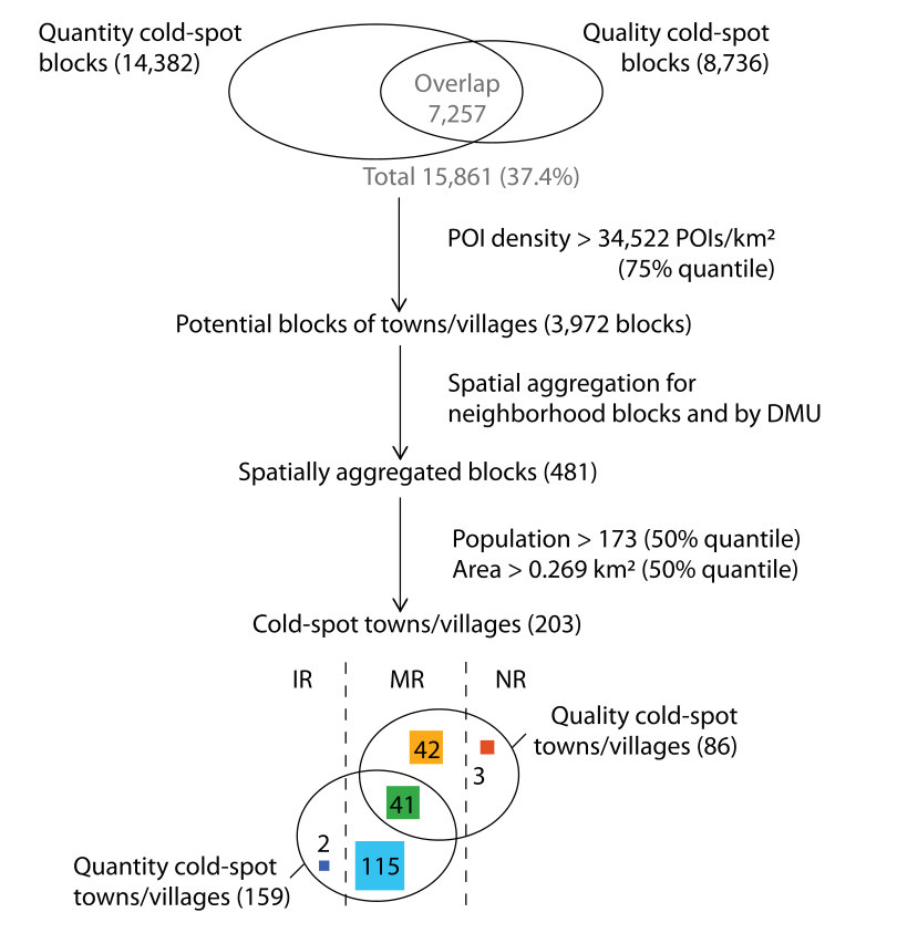
Published reference · STORSTOR paper Fig. 3 — the published town-identification funnel this step
simplifies: 15,861 cold-spot blocks → POI-density filter → spatial aggregation →
population and area thresholds → 203 cold-spot towns/villages, split by DMU stage.
Song et al. (2021), CC BY-NC-ND.
◆How to read this result
The strategy comes from the pair of classes, not from either one. A block that is LL in quantity only needs supply; LL in quality only needs upgrading; LL in both is the joint cold spot. Reading one dimension alone hides which of the three a place is.
Hotspots ring the city rather than covering it. The NR downturn pulls quality back down in the most urban blocks, so they miss the joint hotspot — the trade-off made spatial, and the reason the overlay is worth drawing at all.
Step 5
What each dimension contributes to income (Eq. 10–11)
What this step does
Two models, one question: how much of block income does each dimension explain? The GAM
(mgcv) captures the nonlinear effects; the base-R GWR captures the regional
ones, with its adaptive bandwidth chosen by AICc (k = 80 of 1,600 wins). The
contribution of a dimension is the deviance explained that disappears when it is dropped,
averaged over the two models — the paper's Fig. 11a quantity.
Code
R/50-income-models.R — the entire analytical content of the step
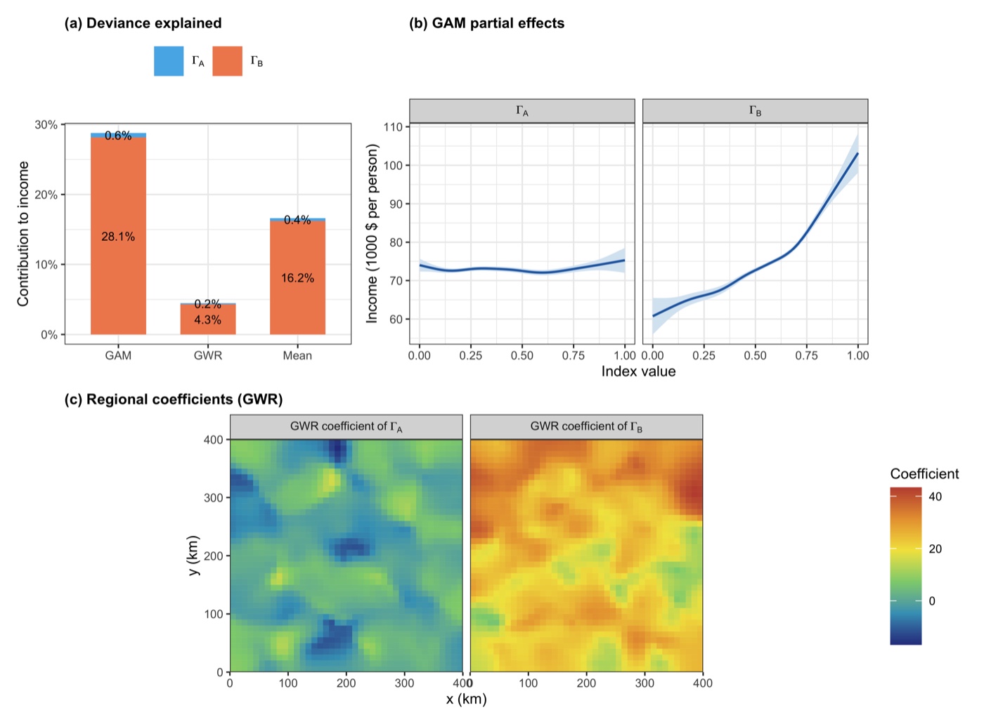
Demo run · fig05Demo fig05 — contribution bars (a), GAM partial effects (b) and GWR
coefficient surfaces (c). Quality dominates income (mean 16.2% vs 0.4%), its partial
effect climbs steeply, and its GWR coefficient grows northward — exactly the drift the
simulation embedded.Published reference · STORSTOR paper Fig. 11 — the published version: ΓB contributes 16.2%
of income against 5.9% for ΓA (a), the joint GAM surface (b), and the GWR
coefficient maps with significance hatching (c–d).
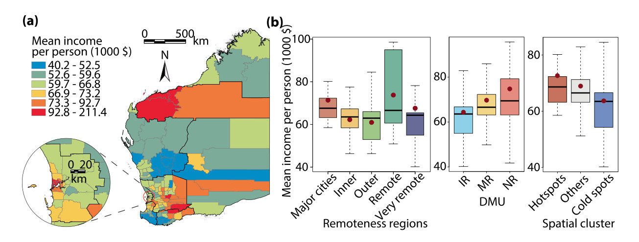
Published reference · STORSTOR paper Fig. 10 — the published response variable: LGA mean income per
person (a), and its relations with remoteness, DMU stage and spatial cluster (b). Income
rises IR → MR → NR, the pattern the contribution analysis then decomposes.
Song et al. (2021), CC BY-NC-ND.
◆How to read this result
Contribution is a drop-one quantity, so the two dimensions need not sum to the total. ΓB explains 28.1% of GAM deviance against ΓA's 0.6%; the remainder is shared between them and cannot be assigned to either.
GWR and GAM disagree in size, not in direction. GWR attributes far less to either dimension (4.3% and 0.2%) because its local intercepts already absorb the regional drift. Averaging the two is deliberate — reporting only the GAM would overstate the effect.
3.4 Reading the Results Together
The three analyses answer one policy question from three sides, and their agreement is the
finding:
DMU stage
Blocks
Share
Mean ΓA
Mean ΓB
Mean Γ
Reading
IR — increase return
205
12.8%
0.058
0.303
0.181
every unit of quantity still buys quality fast: build roads
MR — marginal return
1,162
72.6%
0.299
0.545
0.422
gains flatten: target investment by cluster, not blanket build-out
NR — negative return
233
14.6%
0.698
0.566
0.632
more quantity coincides with declining quality: maintain and upgrade
Demo stage profile (results/dmu-stages.csv, tables/table-dmu-stages.tex).
ΓB rises steeply from IR to MR and then barely — the diminishing margin in one row of numbers.
The curve says when. Quality responds to quantity only below
t1 = 0.092; past t2 = 0.576 the relation turns
negative. The published analogues (0.072, 0.585) put most of Western Australia's remote
blocks in IR and its metropolitan core in NR.
The clusters say where. 242 blocks are cold in both dimensions ("increase both"),
181 only in quantity, 49 only in quality — a budget split, not just a map. The published
overlay (Fig. 8b) reads the same way: 56.7% quantity, 20.7% quality, 20.2% both.
The contribution says why it pays. Income follows quality (16.2%) far more than
quantity (0.4% demo; 5.9% published), and the GWR shows where that payoff is
strongest — northward in the demo by construction, in the remote north of WA in the
published case.
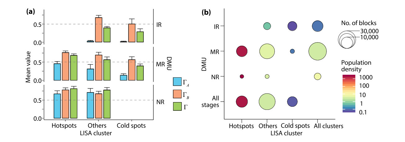
Published reference · STORSTOR paper Fig. 9 — clusters × stages in the published case: cold spots
concentrate in IR and MR, hotspots in MR and NR, and population density tracks the hotspot
column. The demo's cross-tabulation (results/lisa-clusters.csv) shows the same
diagonal.
Song et al. (2021), CC BY-NC-ND.
Category
Dimension
Variable
Entropy weight
density
ΓA
road_density
0.343
main_road_density
0.328
roads_per_person
0.329
connectivity
ΓA
intersection_density
1.000
performance
ΓB
roughness
0.267
rutting
0.260
deflection
0.230
curvature
0.242
safety
ΓB
crash_rate
1.000
accessibility
ΓB
craf_schools
0.310
craf_hospitals
0.352
craf_industry
0.338
transport_modes
ΓB
dist_ports
0.472
dist_airports
0.528
Demo entropy weights (results/entropy-weights.csv) — the analogue of
the paper's Table 2. Weights are near-equal within categories because the simulated
indicators share one latent driver; on real data the spread is informative in itself.
4 Adaptation, Writing & Reproducibility
4.1 Port to Your Domain
STOR is a template for any quantity–quality (or any two-dimension) trade-off measured over
spatial units: hospital beds vs care quality, park area vs park sentiment, water supply vs water
quality, housing stock vs housing condition. Porting is four moves:
1 · Replace the data step
Drop your own
data/blocks.csv and delete R/10-simulate-data.R from
STEPS in run-all.R. One row per spatial unit; coordinates in any
projected CRS.
2 · Declare the indicators
Rewrite
INDICATORS in the config: name, category, dimension (A or B), sign. This table
is your paper's Table 1 — categories decide where entropy weighting happens.
3 · Swap the neighbours
The demo uses
queen contiguity on a grid. For polygons, build the list once with
spdep::poly2nb() and pass it to stor_local_moran() — the neighbour
list is the only spatial input LISA needs.
4 · Re-tune two constants
LOESS_SPAN (see the warning below) and GWR_NEIGHBORS (bracket
~2–10% of your n). Everything else transfers unchanged.
!The span is the one honest judgement call
The DMU boundaries are derivative features of a smoothed curve, and t1 in
particular moves with LOESS_SPAN: too wide and the early rise is flattened into
the axis (t1 slides toward 0), too narrow and η chases noise (spurious boundaries
mid-curve). The demo settled on 0.15 for 1,600 blocks by checking recovery of the embedded
truth — a calibration you cannot run on real data. Report the span, show the utility curve
at two or three spans in a supplement, and treat boundary ranges, not points, as the
policy-safe statement. The t2 = max(u) definition is robust; lean on
it.
✓Sanity checks that transfer to real data
Signs: flip a known-negative indicator and ΓB should drop where that
indicator is bad. If it rises, the sign column is wrong.
Weights: a near-zero entropy weight means a near-constant indicator — decide
deliberately whether it belongs in the index.
Boundaries: t1 < t2 and η > 0 on
(t1, t2) must hold by construction — test-01
checks this shape on any data you feed it.
Clusters: LISA on a permuted response should return almost no significant
blocks; if it does not, the neighbour list is wrong.
4.2 Write the Paper
Every manuscript element of a STOR-style paper maps to a file this pipeline already writes:
Manuscript element
Published analogue
Comes from
Indicator system table (variables, categories, signs)
The result files are the manuscript's skeleton; the writing fills in why each
number matters for the study area.
Manuscript outline
manuscript outline
1  Introduction       — infrastructure is assessed by quantity alone; quality and
                         its trade-off with quantity; the contribution (3 aims)
2  STOR model         — 2.1 The indicator system and its two dimensions
                         2.2 Entropy-weighted indices (Eq. 3–6)
                         2.3 Utility, marginal utility and DMU stages (Eq. 7–9)
                         2.4 Spatial clusters and trade-off strategies
                         2.5 Outcome contribution (Eq. 10–11)
3  Case & data        — study area, block definition, the 14 indicators
4  Results            — 4.1 the two indices across space
                         4.2 the trade-off relation and its stage boundaries
                         4.3 stage profiles and where each stage sits
                         4.4 cold spots and the strategy each one implies
                         4.5 what each dimension contributes to the outcome
5  Discussion         — what the stage boundaries mean for investment; the limits
                         of an entropy-weighted index
6  Conclusions        — the trade-off, its boundaries, and the policy reading
4.3 Final Reproducibility Package
Code
R/02-stor-core.R (the method, base R) + the numbered pipeline + run-all.R + tests/
Data
data/blocks.csv and the embedded truth in data/derived/simulation-truth.csv — or your own blocks table with its provenance
Rscript run-all.R test passes — 25 checks, including that the recovered
boundaries, stages, clusters and contributions match the embedded truth, and that the
local Moran and GWR implementations match their references.
Delete results/, tables/, figs/ and
data/ outputs, re-run Rscript run-all.R — every number and
figure on this page regenerates (~18 s).
The LOESS span, bin count, LISA permutations and alpha, GWR bandwidth candidates and
seed are stated in the manuscript and match config/project-config.R.
The indicator signs of Table 1 are stated with their justification.
env/session-info.txt is included in the deposit.
◆Anticipate the reviewer
Are the DMU boundaries an artefact of the smoothing? → show the curve at two or
three spans; t2 = max(u) barely moves and the stage shares are stable
(§4.1). Why entropy weights rather than expert weights? → they are data-driven and
reproducible; the paper's hierarchy (entropy within categories, equal across) bounds any one
variable's influence. Is quality just a proxy for remoteness? → the GWR separates the
spatial drift from the index effect, and the contribution survives it.
Do the clusters depend on the contiguity choice? → re-run Step 4 with a distance
band; the overlay classes are stable because they require agreement of two dimensions.
Causality? → STOR measures relations and stages; the paper claims strategy relevance,
not causal effects — keep the manuscript's verbs on that side.
References & credits
Demo outputs were generated by the scripts in this folder on simulated data.
Reference figures are reproduced from the cited article for comparison; the STOR
article is open access under CC BY-NC-ND. The implementation follows the article's §3; the
GWR and cold-spot-town departures are described in §2.1 above.
Song Y, Wu P, Hampson K, Anumba C (2021). Assessing block-level sustainable transport
infrastructure development using a spatial trade-off relation model.
International Journal of Applied Earth Observation and Geoinformation 105:102585.
doi:10.1016/j.jag.2021.102585
· PDF
(source of the method and of all reference figures on this page)
Anselin L (1995). Local indicators of spatial association — LISA.
Geographical Analysis 27(2):93–115. (the cluster statistic implemented in
stor_local_moran())
Jacoby WG (2000). Loess: a nonparametric, graphical tool for depicting relationships
between variables. Electoral Studies 19(4):577–613. (the smoother behind
Eq. 7)
Wood SN (2017). Generalized Additive Models: An Introduction with R, 2nd ed.
Chapman & Hall/CRC. (the GAM of Eq. 10, via mgcv)
Fotheringham AS, Brunsdon C, Charlton M (2003). Geographically Weighted Regression.
Wiley. (the model of Eq. 11, re-implemented in base R here)